
Chapter at a glance
Format
Create

Work
Working with custom number formats

Set
IN THIS CHAPTER, YOU WILL LEARN HOW TO
Apply number formatting.
Format with styles.
Create custom themes.
Create custom number and date formats.
Protect worksheets.
Open extra windows in the same workbook.
Most of you have used formatting controls, buttons, and commands, so you’re most likely familiar with fonts and styles. In this chapter, you’ll learn how to format numbers and dates in Microsoft Excel, how to use styles, and how to create custom themes. In addition, you’ll open extra windows in your workbook and use worksheet protection.
It’s been mentioned before, but it bears repeating: formatting does not change the underlying values in cells, even though it may appear to do so. So feel free to experiment. Ctrl+Z (Undo) is your friend.
Practice Files
To complete the exercises in this chapter, you need the practice files contained in the Chapter21 practice file folder. For more information, see Download the practice files in this book’s Introduction.
Formatting is the easiest way to turn a group of numbers into something resembling information, and it really doesn’t take much work to get results.
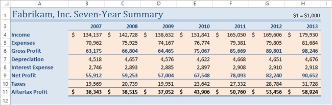
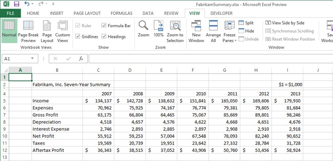
In this exercise, you’ll work with a worksheet that is devoid of formatting, which means that everything is in the General format. Though you may have viewed similar worksheets before, this one is much harder to decipher without formatting.
Set Up
You need the FabrikamSummary_start.xlsx workbook located in the Chapter21 practice file folder to complete this exercise. Open the FabrikamSummary_start.xlsx workbook, and save it as FabrikamSummary.xlsx. Then follow the steps.
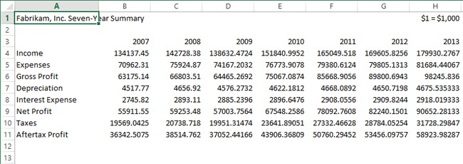
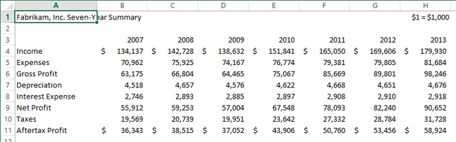
In the FabrikamSummary.xlsx workbook, select all the cells containing numbers (except the dates)—cells B4 to H11.
Click the Comma Style button, located in the Number group, on the Home tab.
All the decimals in the selected cells are rounded to the nearest hundredth.
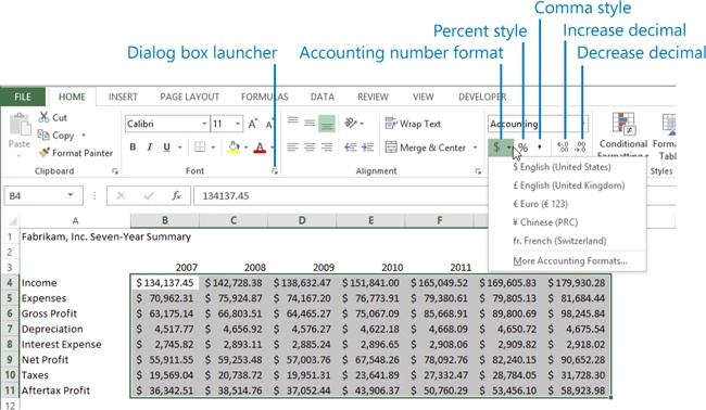
Click the Accounting Number Format button, also in the Number group, on the Home tab, which adds dollar signs to the format.
Click the tiny downward-pointing arrow adjacent to the Accounting Number Format button to display a menu of the same name.
Click fr. French (Switzerland).
Note that changing the currency symbol does not change the values of the numbers (as with all formatting), but notice that the values in row 4 now display a series of pound signs (########), indicating that the contents of those cells are too wide to display. This is because the format adds a space and fr. to the right of each number, which takes up more space in a cell than any of the other currency symbols.
Click the Accounting Number Format button and then click $ English (United States).
Select cells B5:H10 (all the numbers except those for Income and Aftertax Profit). Standard accounting style dictates that dollar signs should only appear in the first and last rows of a table. You don’t necessarily need to follow that rule, but it does make the table a lot easier to read.
Click the Comma Style button (which removes dollar signs from the selected cells).
Select all the cells containing numbers (not dates): B4:H11.
In the Number group, on the Home tab, click the Decrease Decimal button twice.
In a summary worksheet like this, where large sums of money are being reported, pennies are a distraction and don’t need to be displayed.
Click the Center button, in the Alignment group, on the Home tab, and notice that nothing happens; the numbers remain right-aligned. The alignment properties of number formatting override text alignment formatting.
Select the year headings: cells B3:H3.
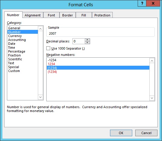
Click the tiny dialog box launcher in the lower-right corner of the Number group, on the Home tab, to display the Format Cells dialog box.
In the Category list, on the Number page, click Number.
In the Decimal places box, enter or select 0.
In the Negative numbers box, click the third option, (1234).
Click OK.
Press Ctrl+Y to redo your changes. Now the date headers line up with the columns.
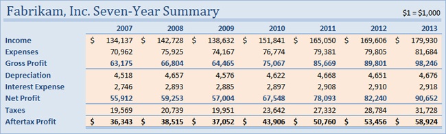
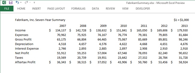
Styles are not always useful in sheets full of numbers, but they can come in handy for more presentation-oriented uses, and of course, if you like the design. Styles can be created by using the regular formatting tools, so if you don’t like something about a style, you can modify it and save it for future reference. Because the numbers were formatted in the previous exercise, let’s continue formatting the sheet.
In this exercise, you’ll apply formatting to the FabrikamSummary worksheet and save it as a style that can be used elsewhere.
Set Up
You need the FabrikamSummary.xlsx workbook you saved at the end of the previous exercise to complete this exercise. Open the FabrikamSummary.xlsx workbook (if it is not already open), and follow the steps.
Select cells A1:I12 (one row deeper and one column wider than the table).
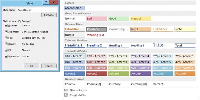
On the Home tab, click the Cell Styles button to display the Styles gallery.
Click 20% - Accent 1.
Select all the numbers below the year headings (cells B4:H11).
Click the Cell Styles button and then click 20% - Accent 6.
Select cell A1.
Click the Cell Styles button and then click Title.
Select all the numbers in the Gross Profit row (cells B6:H6).
Hold down the Ctrl key and select all the numbers in the Net Profit row (cells B9:H9), adding them to the selection.
Click the Cell Styles button and then click Heading 3.
Select all the numbers in the Aftertax Profit row (cells B11:H11).
Click the Cell Styles button and then click Total.
Select the year headers (cells B3:H3).
Click the Cell Styles button and then click Heading 3.
Select all the labels (cells A4:A11).
Click the Cell Styles button and then click Heading 4.
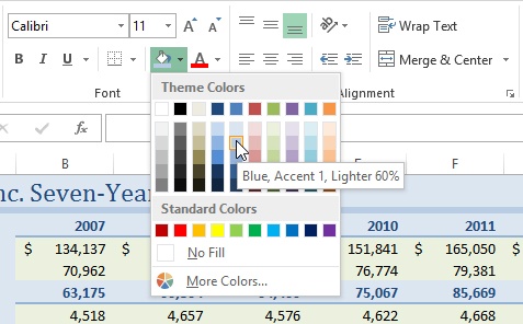
Select the blank cells between the table and the headings (cells A2:H2).
On the Home tab, in the Font group, click the arrow adjacent to the Fill Color button and click a slightly darker shade of blue.
Click cell I2.
On the Home tab, in the Cells group, click the Format button, and then click Row Height.
Enter 5 and press Enter.
Click the Format button, and then click Column Width.
Enter 3 and press Enter.
Click anywhere outside the table and look at the results.
Perhaps it’s not the most beautiful worksheet you’ve ever seen, but it’s certainly easy to read. You can enhance the appearance of the table by modifying fonts, colors, borders, fills, and number formats any way you like. Then you can save the new formats for easy retrieval directly from the Cell Styles menu. Try it.
Click cell A2.
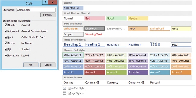
Click the Cell Styles button, and then click the New Cell Style command at the bottom of the gallery.
In the Style name box, enter AccentColor and press Enter.
Now when you click the Cell Styles button, AccentColor appears at the top of the gallery.
Unfortunately, custom formats travel with the workbook and are not even available to other workbooks that might be open at the same time. However, you can use the Merge Styles command located in the lower-left corner of the Cell Styles gallery to propagate custom styles from one open workbook to another. You can also save collections of colors, fonts, and effects as a theme, which we’ll explore next.

When you apply a theme, you change the appearance of everything in the workbook, regardless of what is currently selected. Themes are made up of colors, fonts, and effects. They do not apply number, alignment, or protection formats. Themes are not workbook dependent. When you save a custom theme, it is available to use with other workbooks, and it’s also available for use in other Office applications.
In this exercise, you’ll apply a theme, then modify it, and then save it as a new theme.
Set Up
You need the FabrikamSummaryTheme_start.xlsx workbook located in the Chapter21 practice file folder to complete this exercise. Open the FabrikamSummaryTheme_start.xlsx workbook, and save it as FabrikamSummaryTheme.xlsx.
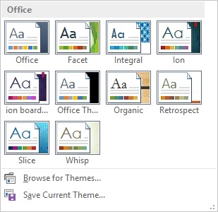
In the FabrikamSummaryTheme.xlsx workbook, click the Page Layout tab and then click the Themes button.
Point to a theme in the gallery to display a preview on the worksheet. Because this table was formatted by using cell styles, all the fonts and colors used in the table change according to the selected theme (along with effects, if any graphic objects were present).
Click the Integral theme.
Important
Software continues to be updated long after books are published, and newer versions of Excel may offer a somewhat different selection of themes, color sets, font sets, and effects. Installed fonts vary from system to system, and any themes that you or members of your workgroup created with Excel or any other Office application may also be visible. Use whatever is available (or whatever you prefer).
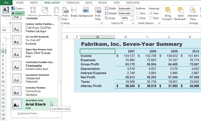
On the Page Layout tab, in the Themes group, click the Colors button. (Point to various color sets to preview their effects.)
Click the Blue Green color set.
In the Themes group, click the Fonts button. (Point to various font sets to preview their effects.)
Scroll down the list and click the Arial Black font set (or your favorite, if Arial Black is not available on your system).
In the Themes group, on the Page Layout tab, click the Themes button and then click Save Current Theme at the bottom of the gallery. You’ll notice that the default folder is the MicrosoftTemplatesDocument Themes folder, a global settings folder that is available to other Office applications.
Enter Fabrikam1 in the File name box.
Click Save.
Click the Themes button again, and the Fabrikam1 theme appears at the top of the gallery, beneath the Custom heading.
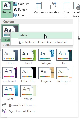
You can create as many themes as you want, and you can add themes from other disk or network locations by using the Browse For Themes command located in the lower-left corner of the Themes gallery. If you later decide you don’t want to keep it, it’s easy to delete a custom theme.
Click the Themes button.
In the Themes gallery, right-click the Fabrikam1 theme to display a shortcut menu.
If you want to remove a custom theme, click Delete to remove it from both the Themes gallery and the Document Themes folder. But make sure this theme isn’t in use in other workbooks or other Office documents.
Press the Esc key.

This is a little-used feature that went largely unnoticed when it appeared in a previous version of Excel. Prior to that version, it was possible to apply formatting only to the entire contents of a cell, but today, you can format individual characters within a cell. This is a useful feature when you are organizing workbooks and trying to fit into the cell structure with linear content like headings and paragraphs of text.
In this exercise, you’ll apply formatting to individual characters in a cell.
Set Up
You need the FabrikamSummaryTheme.xlsx workbook you saved at the end of the previous exercise to complete this exercise. Open the FabrikamSummaryTheme.xlsx workbook (if it is not already open), and follow the steps.
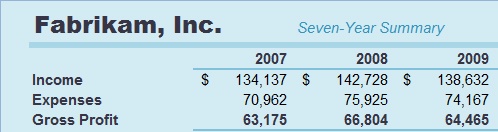
Double-click cell G1.
A flashing text cursor appears in the cell.
Drag through the words Seven Year Summary to select them.
A small floating toolbar called the mini toolbar appears. You can use this toolbar to edit the selected text (or you can use the tools in the Font group, on the Home tab).
Select Arial from the Font list.
Reduce the font size to 11.
Click the Italic button.
Change the font color to your favorite theme color (we chose Aqua).
Click anywhere outside the table to view the changes.

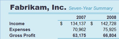
Individuals who have used Excel for a long time (before in-cell formatting was possible) might attempt to put Fabrikam, Inc. and Seven-Year Summary into two separate cells and then apply formats to each cell individually. That process works, too, but the cells won’t line up correctly. The result will look something like the text in the following graphic.
Custom number formats are like programming code; very easy programming code. Excel has its own number-formatting language. Every built-in number format can be expressed by using code, and thus can be easily modified for your own purposes.
In this exercise, you’ll work with some of these formatting codes.
Set Up
You don’t need any practice files to complete this exercise. Open a blank workbook and follow the steps.
Select cells A1:A4.
Click the Accounting Number Format button ($) on the Home tab.
Press Ctrl+1 to display the Format Cells dialog box (or click the dialog box launcher in the Number group on the Home tab).
Click the Number tab, if it is not already active.
Click the Custom category.
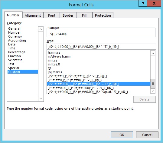
The following table further describes the code behind the format applied by using the Accounting Number Format button. You can view the code behind any format in the Format Cells dialog box, in the Category list, by first clicking the category and then selecting the format you want to use. Then click the Custom category. The code for the currently selected format is displayed in the Type box, and it is editable. You cannot overwrite a built-in code, so if you edit a code and click OK, a new code is added to the Type list and is available the next time you open the Format Cells dialog box.
We created a modified version of the Accounting Number Format code, as shown in the following table. Format codes have four components separated by semicolons:
($* #,##0.00_);_($* (#,##0.00);_($* "-"??_);_(@_)Values
Positive
Negative
Zero
Text
Code
_($* #,##0.00_)_($* (#,##0.00)_($* "-"??_)_(@_)Entered
1234-12340Hello!Displayed
$ 1,234.00$ (1,234.00)$ -Hello!Click OK to exit the dialog box.
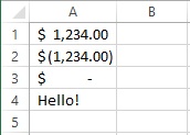
Click cell A1. Enter 1234 and press Enter.
In cell A2, enter -1234 and press Enter.
In Cell A3, enter 0 and press Enter.
In cell A4, enter Hello! and press Enter.
Select cells A1:A4.
Press Ctrl+1 to display the Format Cells dialog box (or click the dialog box launcher on the Home tab, in the Number group).
Click the Custom category.
In the Type box, replace the dash (–) in the third section of the format code with the word Zero. Be careful not to delete the quotation marks.
Click OK.
If you were wondering why they went to the trouble of specifying codes for the text section of the Accounting Number format, because text would display anyway, you’ll notice that Hello! lines up perfectly with the dollar signs, which would not be the case without the special code. Details matter.
Tip
You can create a formatting code that explicitly excludes one or more of the four value types from being displayed. For example, simply delete everything after the third semicolon (but not the semicolon itself) in the Accounting Number Format code to hide all text entries. The code 0.00;;; displays only positive numbers and hides everything else. And the handy ;;;; (four semicolons) code hides everything. You might use this trick to hide a formula on the worksheet; the result of which you need to use elsewhere, but don’t need to display.
Following are the descriptions of the formatting codes that were used in the table shown previously:
Underscore (_). Adds an invisible space that is exactly the same width as the character immediately following it. Each section in the previous code begins with an underscore and an opening parenthesis. (This adds a parenthesis-sized space before anything else in the cell, for visual balance. In all but the negative values section, there is a matching underscore at the end of the code section. This adds a balancing blank space on the right side of the cell. Negative values are, of course, surrounded by fully visible parentheses. Adding these spaces allows positive and negative numbers to be correctly aligned in a column.
Asterisk (*). The character immediately following is to be repeated sufficiently to fill the column width. So, in this case, the dollar sign always stays on the left side of the cell, with as many spaces added between it and the number as necessary.
Zero (0). This is a required digit placeholder. If there are no other digits to display in that position, Excel will always display zeros.
Pound sign (#). This is an optional digit placeholder; if there is no digit in that position, it remains blank.
Question mark (?). This is a required spaceholder. Even if there are no other digits to display in that position, Excel will always add a space. It is employed in the previous code to add two spaces after the dash, corresponding to two decimal places. This ensures that dashes (indicating zero values) will always line up with decimal points in a column of otherwise-nonzero numbers.
Quotation marks (” “). These indicate a text component. In the code created previously, a dash is enclosed in quotation marks in the zero values position. In the accounting formats, only a dash is displayed if an entry equals zero.
At symbol (@). This is a text placeholder, similar to the # that is a number placeholder. If there is text in the cell, it is displayed at this position.
Comma (,). Otherwise known as a comma separator, this tells Excel to add commas to separate numbers, such as thousands, millions, and so on. It can also be used to apply gross rounding and scaling. For example, the format code #,###,### would display 4567890 as 4,567,890, but if you apply the code #,###, to the same number, the cell displays the number as 4,568. This kind of rounding/scaling can be used to make reports easier to read when they’re displaying numbers in the millions and billions.
Select cell D1.
Press Ctrl+1 to display the Format Cells dialog box (or click the dialog box launcher on the Home tab, in the Number group).
Click the Special category and click Social Security Number.
Click the Custom category to view the custom formatting code 000-00-0000, which is used to format social security numbers.
If you go back to the Special category and click either of the Zip code options, similar codes appear that are made up of zeros (and dashes). This indicates that each of these format codes will correctly display the exact number of digits indicated, and if no digit exists, a zero is displayed.
Click the Special category, select Phone Number, and click OK to apply the format to cell D1.
Press Ctrl+1 and click the Custom category.
Tip
When you create a custom format, it is saved with the workbook and remains available in the Format Cells dialog box’s Custom category. If you want to use it elsewhere, you can copy a formatted cell from one workbook to another; the custom format travels with it.
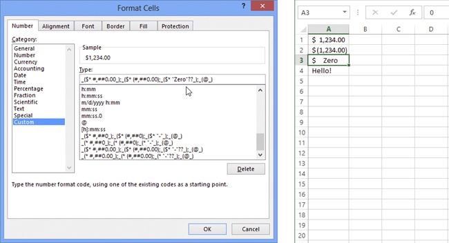
Let’s take a closer look at this formatting code in the following table. Notice that it has only two sections separated by a semicolon. This would seem to indicate that only positive and negative numbers are specified in this code, but actually, because there is a comparison operator (<=) involved, the semicolon is used to specify an either/or alternative. If the condition specified in the first section does not apply, then the second section is used.
See Also
For information about Excel’s Conditional Formatting command that allows you to easily apply selective formatting depending on the contents of the cells, see Chapter 20.
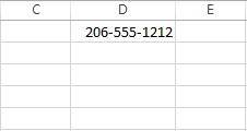
[<=9999999]###-####;(###) ###-####Values
Condition 1
Condition 2
Code
[<=9999999]###-####(###) ###-####Entered
55512122065551212Displayed
555-1212(206) 555-1212This is a clever code. The bracketed comparison value eliminates anything larger than 7 digits, displaying only phone numbers that do not include area codes. If the number entered is larger than 7 digits, the second section of the formatting code takes over and adds parentheses around the first three numbers. Let’s modify it.
Edit the second section of the code in the Type box as follows (delete the first parenthesis and replace the second one with a dash):
[<=9999999]###-####;###-###-####
Click OK.
Enter 2065551212 and press Enter.
Custom formats remain available for use in the workbook in which they were created during the current session. However, if you save the workbook without actually applying a custom format to any values, it will not be available the next time you open the workbook. These are all good reasons to keep track of the custom formats you want to keep.
Tip
For more information about using operators in formatting codes, click the Help button in the upper-right corner of the Excel window and enter custom number format into the search box. In the topic Create Or Delete A Custom Number Format, scroll down to Guidelines For Using Decimal Places, Spaces, Colors, And Conditions.
Note that the special Phone Number code will display as many numbers as you enter the digits for (unlike the social security number and ZIP code formats, which always display the same number of digits, adding leading zeros if necessary). For example, if you were to enter an incorrect numbers of digits into cells formatted with the Phone Number code, the numbers will be displayed as entered, such as in 23-4567 or (12) 345-6789 or (1234) 567-8909. Leading zeros are ignored in the Phone Number code, but not in the other Special codes.
Tip
You can add bracketed conditions such as [<=9999999] to any formatting code, but be aware that when you use conditions, the usual four-part positive-negative-zero-text code structure changes to condition1-condition2-condition3, where the optional condition3 is essentially the else condition to be applied if the first two conditions are not met. If you still want to control negative values, then you can manually add the [<0] operator to the second condition.
When you apply a percentage format to a number, Excel essentially moves the decimal point two places to the right, adds a percent sign, and rounds to a specified number of decimal places (depending on the format selected). For example, if a cell contains the number .3456 and you format it by clicking the Percent Style button (which applies a percentage format with no decimal places), Excel displays 35% in the cell.
Note this fact about percentage formats: after you apply one, Excel assumes there should be a decimal point even if you don’t enter one. So, if you want to change the percentage in that same cell to 38%, you can just enter 38 (which is really 3800%) rather than .38. Microsoft learned that when changing a number displayed as a percentage, most people just enter an integer, not a decimal, so they made the format smart enough to deal with it. But, of course, if you really meant to enter 3800% when you entered 38, you’ll have to go back and enter 3800.
There’s not much you need to modify with percentages. You just need to decide whether or not you want to display decimals. You can display up to 30 decimal places. You can also add custom formatting. In this exercise, you’ll do both.
Set Up
You need either the Custom Formats.xlsx workbook you saved at the end of the previous exercise or the Custom Formats_start.xlsx workbook located in the Chapter21 practice file folder to complete this exercise. If you are using the Custom Formats_start.xlsx workbook, open it and save it as Custom Formats.xlsx.
In the Custom Formats.xlsx workbook, click the New Sheet button next to the Sheet1 tab at the bottom of the workbook window to create a new worksheet. You will save the custom formats from each exercise on a separate sheet in this workbook.
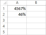
In cell A1, enter 45.67 and press Enter.
Select cells A1:A2.
On the Home tab, in the Number group, click the Percent Style button.
Select cell A2.
Enter 45.67 and press Enter.
Notice the difference between applying the format before or after entering values. Most of the time, you’ll apply percentage formats to cells containing formulas that generate actual percentages, but if not, check the values after applying a percentage format to a large range of cells containing existing values.
Select cell A1, enter 45.67, and then press Enter.
Select cells A1:A2.
Press Ctrl+1 to display the Format Number dialog box, and notice that Decimal Places is the only option you can change in the Percentage category.
Click the Custom category.
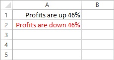
In the Type box, replace the existing code (0%) with the following:
“Profits are up “0%;[Red][<0]”Profits are down “0%
Press Enter.
Enter -45.67 into cell A2
Press Enter.
If you want the look of fractions and do not require the precision of decimals, Excel offers formatting options that allow plenty of control over their display. However, you may need to adjust fraction formats to suit your needs. Though fraction formats often apply a rounding factor to the actual value in the cell (unless there is no remainder, or MOD value), doing so changes the display, but as always, does not alter the underlying value.
In this exercise, you’ll apply fraction formatting and work around some of its idiosyncrasies.
Set Up
You need either the Custom Formats.xlsx workbook you saved at the end of the previous exercise or the Custom Formats 2_start.xlsx workbook located in the Chapter21 practice file folder to complete this exercise. If you are using the Custom Formats 2_start.xlsx workbook, open it and save it as Custom Formats.xlsx.
In the Custom Formats.xlsx workbook, click the New Sheet button next to the sheet tabs at the bottom of the workbook window to create a new worksheet. You will save the custom formats from each exercise on a separate sheet in this workbook.
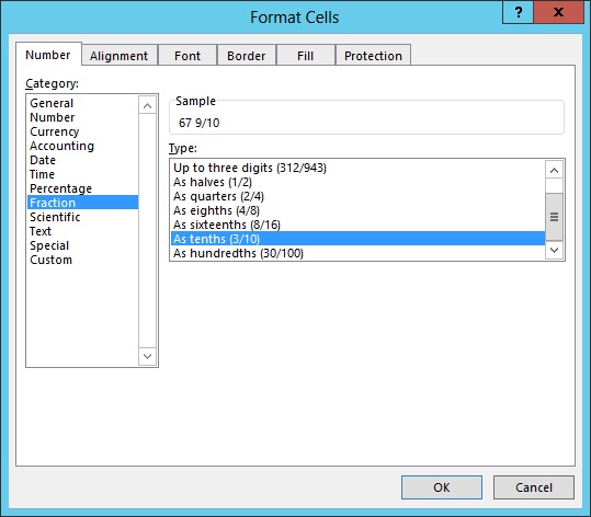
Select cell A1.
On the Home tab, in the Number group, click the Number list and select Fraction.
The fraction displayed in the cell uses a denominator (9) not commonly used in fractions. This may be the closest actual fractional value (67.8888...), but we need to adjust our fraction so that it uses a more conventional denominator.
Press Ctrl+1 to display the Format Cells dialog box.
In the Type list, scroll down to the bottom.
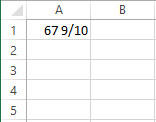
Select As tenths (3/10).
Click OK.
There are a number of fraction formats available, some of which seem barely usable. Consider the Up To Three Digits (312/943) format, which would actually raise precision considerably, while equally reducing intelligibility and making the use of decimals seem more prudent. But the essential options are all here: Halves, Quarters, Eighths, Sixteenths, and Hundredths. But what if you need a few more?
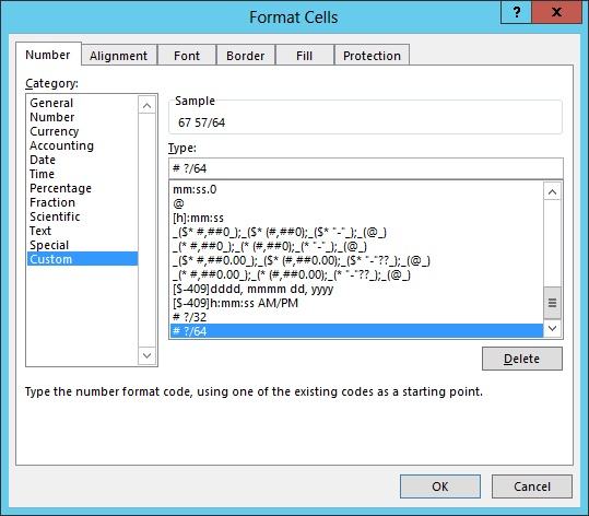
Select cell A1, and then press Ctrl+1 to display the Format Cells dialog box.
Click the Custom category.
In the Type box, replace the existing code (# ?/10) with the following:
# ?/32.
Click OK.
Press Ctrl+1 to open the Format Cells dialog box again.
Click the Custom category.
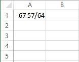
In the Type box, replace the existing code with the following:
# ?/64.
Click OK.
When you open the Format Cells dialog box, the two formats you just created appear somewhere in the list of Custom formats. These two happen to show up at the bottom.


Excel stores dates as serial numeric values starting from January 1, 1900; each day counts as 1. For example, this sentence was written at around 41182.66937 (decimal values, as you might guess, indicate exact time of day), otherwise known as 4:03 P.M. on September 30, 2012. This numeric date system allows you to manipulate dates and times in Excel as easily as other numbers. The time and date formatting options and their associated codes are appropriately different from any of the others.
In this exercise, you’ll apply date formatting and create custom date formats.
Set Up
You need either the Custom Formats.xlsx workbook you saved at the end of the previous exercise or the Custom Formats 3_start.xlsx workbook located in the Chapter21 practice file folder to complete this exercise. If you are using the Custom Formats 3_start.xlsx workbook, open it and save it as Custom Formats.xlsx.
In the Custom Formats.xlsx workbook, click the New Sheet button next to the sheet tabs at the bottom of the workbook window to create a new worksheet. You will save the custom formats from each exercise on a separate sheet in this workbook.
In cell A1, enter 41182.66937, and then press Enter.
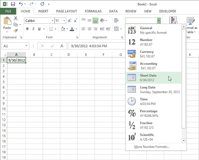
Select cell A1, click the Number drop-down list on the Home tab, and then click Short Date.
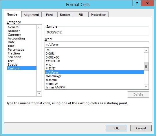
Press Ctrl+1 to display the Format Cells dialog box.
Click the Custom category.
In the Type box, replace the selected formatting code m/d/yyyy as follows:
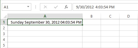
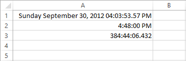
dddd mmmm dd, yyyy hh:mm:ss am/pm
Click OK.
The format now spells out months and days, and includes hours, minutes, and seconds. But if you were timing races or scientific experiments, you might need even more precision.
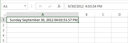
Press Ctrl+1 again to display the Format Cells dialog box.
Make sure the Custom category is still active, and edit your custom formatting code, adding .00 after the seconds, as follows:
dddd mmmm dd, yyyy hh:mm:ss.00 am/pm
Click OK.
Because the time component now includes fractional seconds, this moment in time actually occurred a few hundredths of a second earlier.
In cell A2, enter 41198.7, and then press Enter.
Reselect cell A2, click the Number list on the Home tab, and then click Time.
Cell A2 displays only the time of day represented by the number you entered.
With cell A2 selected, look in the formula bar. The full date and time is displayed there, rather than the number that you entered. The underlying value is still there. This is an aspect of Excel formatting that’s quite helpful. If you really need to view that serial value again, apply the General format from the Number Format list. (If you did this, press Ctrl+Z to undo before proceeding.)
Select cell A3, enter =A2-A1 and press Enter.
This simple formula returns a result that is formatted as a time value, similar to cell A2. (Excel adds formatting to an unformatted cell containing a formula that refers to formatted values.)
Reselect cell A3, click the Number Format list on the Home tab, and select Long Date.
Excel reveals the date Monday, January 16, 1900. This rather cryptically reveals the number of days that have elapsed between the two dates in the formula (16 days, given that 1/1/1900 is day 1). However, in this case, the desired outcome is to display elapsed time.
Press Ctrl+1 to open the Format Cells dialog box.
Click the Custom category.
Replace the formatting code in the Type box with the following:
[hh]:mm:ss.000
Click OK. Now the elapsed time is 384 hours (16 days), 44 hours, and 6.432 seconds.
See Also
For more information about using functions in Excel to calculate dates, see Chapter 19.
When you add brackets around the first component of a time format, Excel returns elapsed time. The brackets must be around the first component only; they will not work in any other position. However, you can change the code to show only elapsed minutes by deleting [hh]: and adding brackets around mm instead. Or, you can use the code [ss] to show only elapsed seconds. The code .000 appended to the seconds component of the format adds precision down to milliseconds (thousandths of a second), which is as precise as Excel will go. You can’t add more than three zeros to the code.

Following is a list with descriptions for several date formatting codes:
d (Day). This code displays either numbers or text, depending on how many of them you include in the format. A single d displays the date as a number without leading zeros (1 or 16). A double dd displays the date as a number with leading zeros (01 or 16). Instead of displaying a date, using a triple ddd code displays the name of the day of the week, abbreviated (Sat). Similarly, using a quadruple dddd code displays the full name of the day of the week (Saturday). You can use both numeric dates and day names in formats. For example, a cell containing the date 12/6/2013 that is subsequently formatted using the code dddd mmmm d displays Friday December 6.
m (Month). Like the day code, the month code displays either numbers or text, depending on how many you include in the format. A single m displays the month as a number without leading zeros (1 or 12). A double mm displays the month as a number with leading zeros (01 or 12). The triple mmm code displays an abbreviated month name (Dec). A quadruple mmmm code displays the full name of the month (December). (See also mm (Minutes), later in this list.)
y (Year). You can use the code yy to display just the last two digits of the year (13), or use yyyy to display the full year (2013).
h (Hour). There are two ways to use the hour code: h displays the hour without leading zeros (2, 22), while the code hh displays the hour with leading zeros (02, 22). Note that Excel always uses a 24-hour clock unless you add the am/pm code.
mm (Minutes). Obviously, minutes and months use the same code letter (m), so it’s all about where you put them. In a date code, the m stands for months, in a time code (separated by colons), it’s minutes. A single m displays minutes without leading zeros (5, 55), while the double mm displays minutes with leading zeros (05, 55).
s (Seconds). A single s displays seconds without leading zeros (3, 33), and a double ss displays seconds with leading zeros (03, 33). Adding a period and one or two zeros to the end of a seconds code (s.0, ss.0, s.00, or ss.00) adds tenths or hundredths of a second to the display, respectively.
am/pm or a/p. Adding am/pm to the end of a date or time format code instructs Excel to display the time component based on a 12-hour clock. Case doesn’t matter.
[ ] (Brackets). Brackets around a time code tell Excel to return elapsed time rather than actual time. It is necessary to apply this format to formulas that calculate elapsed time, otherwise the results may not be what you expect. You can only use brackets with time codes, and only in the first section of the code, for example [hh]:mm:ss or [mm]:ss.
There are some code combinations that won’t work. For example, you cannot use the am/pm format code with a bracketed elapsed-time code, which makes sense if you think about it. Mixing date codes and numeric format codes doesn’t work, either. Feel free to experiment; Excel will let you know what doesn’t work by displaying an error message if you try to create an unusable code.
You and I might not think of protection as a format, but Excel does. You can use it like a format in the sense that you can apply it to some cells and not others. This allows you to lock all the cells in a worksheet to protect them from modification, or you can leave specific cells unlocked, allowing users of the workbook to enter data, and allowing you to specify exactly which areas in the worksheet you want to protect.
Excel assumes that you want to lock all the cells in a workbook if and when you activate protection, so all cells are formatted as locked by default.
In this exercise, you’ll work with protection formatting by unlocking cells on a worksheet that you want to be able to edit after protection is turned on.
Set Up
You need the Real-Estate-Transition_start.xlsx workbook located in the Chapter21 practice file folder to complete this exercise. Open the Real-Estate-Transition_start.xlsx workbook, and save it as Real-Estate-Transition.xlsx.
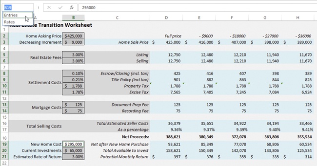
In the Real-Estate-Transition.xlsx workbook, click the arrow next to the Name box in the Formula bar, and select the name Entries to select all the user-input cells in column B.
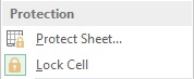
Click the Format button, on the Home tab, and take a look at the Lock Cell command.
The icon adjacent to the Lock Cell command is enclosed in a gray box, which indicates that it is currently active, or locked, as is the case with all cells in a worksheet unless you specify otherwise.
Click the Lock Cell command to unlock the selected cells.
Click the Format button again, and this time, click the Protect Sheet command to display a dialog box of the same name.
You’ll notice that the only allowed default settings involve selecting cells, unless you click additional options.
Click OK to turn on sheet protection without adding a password or selecting additional options.
Select cell B3.
Enter 8000 and then press Enter; Excel accepts the entry and B4 becomes the active cell.
When you try to enter anything into a cell other than those you unlocked in column B, Excel prevents any entry and displays a warning message.

You can protect formulas and data on worksheets that you need to share with others by using protection formatting. Or you can lock all cells on a sheet and optionally apply a password to prevent any changes from happening at all. Protection is applied per worksheet, so a workbook may contain both protected and unprotected sheets.
Protecting workbooks
Protection in Excel has many levels. You protected cells and sheets, so to display the various options for workbook protection, click the File tab to display the Backstage view, click Info, and then click the Protect Workbook button.
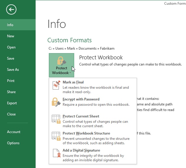
Mark as Final. Makes the workbook read-only
Encrypt with Password. Displays a dialog box allowing you to specify a password necessary to open the workbook
Protect Current Sheet. Prevents the editing of any locked cells on the current sheet and displays the same Protect Sheet dialog box shown earlier in this chapter, with which you specify allowable editing actions for the current sheet
Protect Workbook Structure. Allows you to open workbooks and edit worksheets, but not to rename tabs or move, hide, or unhide worksheets and windows
Add a Digital Signature. Allows you to apply authentication to a workbook by using a digital stamp, which you must purchase from an authorized digital certificate–issuing authority such as Verisign
When creating workbooks designed for presentation, you can control a variety of display settings by using commands on the View tab. The ribbon and controls of the Excel program and the workbook structure can be a distraction in themselves. Some of these settings are saved with the workbook, and thus can for all intents and purposes be considered among your formatting options. We’ll start with the simplest worksheet imaginable to illustrate the remarkable amount of visual clutter you can eliminate if you want to.
In this exercise, you’ll change the way your worksheet is displayed on screen.
Set Up
You need the FabrikamSummary2_start.xlsx workbook located in the Chapter21 practice file folder to complete this exercise. Open the Fabrikam-Summary2_start.xlsx workbook, and save it as FabrikamSummary2.xlsx.
With the FabrikamSummary2.xlsx workbook open, click the View tab.
On the View tab, in the Show group, clear the Gridlines, Headings, and Formula Bar check boxes to deselect those options.
Double-click the View tab to collapse the ribbon and transform the tabs into a menu bar.
Click the Ribbon Display Options button, located in the upper-right corner of the screen, and click the Auto-Hide Ribbon command, which hides the ribbon and the status bar, maximizes the window and hides the Quick Access Toolbar and the tabs. (The formula bar and headings would be visible in this display mode if you hadn’t already turned them off on the View tab.)
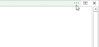
Click the ... (three dots) in the upper-right corner of the screen to temporarily display the ribbon.
Click the Ribbon Display Options button again and click Show Tabs to redisplay the tab names, the status bar, and the Quick Access Toolbar. The ribbon is still hidden.
Click the View tab to temporarily redisplay the ribbon.
When you click a collapsed tab, it appears and stays visible until you click a command or click in the worksheet area.
Click anywhere in the worksheet area. The ribbon collapses again.
Double-click the View tab to redisplay the ribbon (or you can click Ribbon Display Options, and then click Show Tabs and Commands).
Tip
You can double-click any ribbon tab to toggle the ribbon display on or off. If the ribbon is visible, double-clicking any tab hides it; if the ribbon is not visible, double-clicking any tab redisplays it.
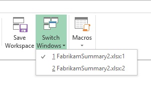
You can create another view of a worksheet by using the New Window command on the View tab. This creates not another worksheet, but another window on the same worksheet, within which you can have an entirely different set of view options, regardless of whether the ribbon is collapsed.
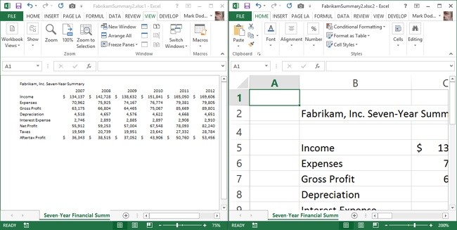
Click the New Window command on the View tab; a new window appears entitled FabrikamSummary2.xlsx:2, displayed with the default View settings.
Click the Zoom button on the View tab, select 200% and click OK.
Click the Switch Windows button and select the unchecked window (FabrikamSummary2.xlsx:1).
Click the Zoom button, select 75% and click OK.
Click the Arrange All button, and accept the default Tiled option.
Click OK.
Tip
You can click the View Side By Side button to do a row-by-row comparison of two workbooks or windows together onscreen. (If you have more than two workbooks or windows open, a dialog box appears allowing you to select one.) When you click the View Side By Side button, the Synchronous Scrolling button is engaged as well. If you want, click the Synchronous Scrolling button to turn it off, and scroll freely in either window.
Many of the settings you select on the View tab are saved with the workbook, including the display of gridlines, headings, and Zoom settings. When you save the workbook with any of these options changed, they persist the next time you open the workbook, including any additional windows created using the New Window command. However, you cannot save the layout of windows, such as the Tiled layout just discussed. But the windows are there, saved with the workbook; you’ll just have to use the Arrange All command again to reset the layout. This is something you can’t do in Excel 2013 that you used to be able to do. As a byproduct of the Single-Document Interface, the Save Workspace command had to be removed, because new windows are no longer contained within a workbook-specific workspace, but now are created in an entirely separate instance of Excel.
Tip
You lose a lot of screen real estate with multiple windows open and a ribbon and Formula bar in each one. Click the Formula bar option on the View tab to hide it. Double-click any tab to collapse the ribbon (double-click the tab again to restore it).
Collapsing the ribbon and hiding the Formula bar are application settings that are not saved with workbooks. The configuration in place when you exit is displayed the next time you start Excel.

If you go to the trouble of creating beautiful and useful worksheets, chances are you would like to use them again, or at least repurpose parts of them. Custom formats you create only apply to the workbook in which you created them. But you can transfer them by copying custom-formatted cells and pasting them into other workbooks. So, you could create a boilerplate workbook to store your number formats created by using custom codes, as well as cell formats, tables, and so on. Or you can create a template. In addition, you can also store workbooks and formats in a location where you can easily retrieve a copy.
Tip
You can save specific formatting options (fonts, colors, and effects) as themes, which can be easily used in other Excel workbooks as well as in other Office documents. See Creating custom themes, earlier in this chapter.
If you have created and used templates in Office applications before, the procedure for saving and accessing templates works a bit differently in Office Home and Student 2013. Before you save your own templates, you need to first specify a Default Personal Templates Location. In order to do this properly, you need to create it first. So before you do anything else, open File Explorer and create a folder to store templates on your computer in a location of your choice. You can place a copy of a random Excel workbook in there too, if you want.
In this exercise, you’ll save a workbook as a template.
Set Up
You don’t need any practice files to complete this exercise. Start Excel, open a blank workbook, and follow the steps.
Click the File tab and then click Options to display the Excel Options dialog box.
Click the Save category.
In the Default Personal Templates Location box, enter the path to the folder you will use to store your templates (or for now, you can copy whatever is in the Default Local File Location box and edit it later).
Click OK.
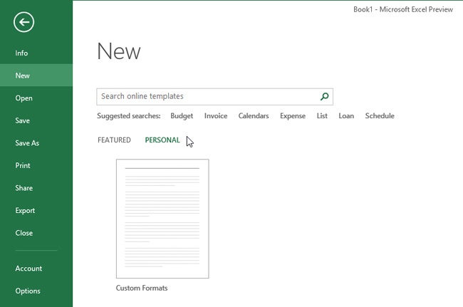
Click the File tab, and then click New.
On the New page, next to Featured, which previously stood alone, there is now a Personal category. When you click this category, any templates stored in your designated personal templates folder are displayed on the screen for you to open with a single click. (We added one for the purposes of this discussion; otherwise, the Personal category would not appear at all unless there was a subfolder in your Default Personal Templates folder.) As a matter of fact, any Excel workbooks stored in this folder will be presented as options in the Personal template category and will open as templates, whether or not you save them as such.
You can create as many templates as you choose, from workbooks containing only custom number formats to fully developed applications, and you can store them in your Default Personal Templates Location. When you open any workbook from the New page of the Backstage view, a copy is opened in Excel, using the original filename with an appended number. For example, a workbook or template named Custom Formats would open as Custom Formats1, which makes it harder to inadvertently overwrite the original file.
When you save a workbook created from a template, the Default Local File Location (specified in the Excel Options dialog box) is offered as the default folder, rather that the Default Personal Templates Location, which further protects the original file from being overwritten.
Formatting helps transform raw numeric data into more accessible information.
You can format cells, and you can format individual characters in cells.
You can modify and create your own variations of Excel’s built-in number formats.
You can modify and create your own date formats, including special elapsed-time formats.
Styles and themes are collections of formatting options that help you maintain consistency among documents.
You can selectively apply protection formatting to lock and unlock individual cells, allowing you to ensure the integrity of formatting and critical formulas on the worksheet.
You can open more than one window on the same workbook, and you can arrange all the open workbooks and windows onscreen for simultaneous viewing.
You can store your formatting choices as templates, making them available for easy duplication.