
Chapter at a glance
Freeze
Freeze worksheet panes so that you always know where you are, Set Up
Print specific rows and columns on every page of output, Printing row and column labels on every page
Break
Break your printed pages by dragging borders in Page Break Preview, Adjusting page breaks
Drag
Drag worksheets between workbooks, Manipulating sheets

IN THIS CHAPTER, YOU WILL LEARN HOW TO
Use Excel’s table features to insert and delete rows and columns.
Keep row and column labels in view, in print and on screen.
Adjust page breaks.
Create and work with multisheet workbooks.
Create multisheet formulas.
Arrange workbooks and windows on screen.
Regardless of what you plan to put in them, it’s important to know the basics of workbooks and worksheets. How do they actually work? Being able to to manipulate the structure of your workbooks may change your thinking about how to organize your data.
In this chapter, you’ll learn how to insert and delete cells, rows, and columns; how to change display and print options; and how to use multiple sheets in a workbook.
Practice Files
To complete the exercises in this chapter, you need the practice files contained in the Chapter22 practice file folder. For more information, see Download the practice files in this book’s Introduction.
There are certain actions that accrue more usage in applications. Like copying and pasting in Microsoft Word, inserting and deleting rows and columns in Microsoft Excel is near the top of that list.
In this exercise, you’ll insert some rows and add a column of totals with the help of Excel’s table features. But first, you’ll sort the existing worksheet.
Set Up
You need the FabrikamQ1_start.xlsx workbook located in the Chapter22 practice file folder to complete this exercise. Open the FabrikamQ1_start.xlsx workbook, save it as FabrikamQ1.xlsx, and then follow the steps.
With the FabrikamQ1_start.xlsx workbook open, make sure that cell A2 is selected, and then click the Data tab.
Click the Sort button in the Sort & Filter group.
Because the active cell is in a table, Excel automatically selects the entire table when the Sort dialog box appears.
In the Sort by list, select Group.
Click the Add Level button.
In the Then by list, select Channel.
Click OK to sort the table.
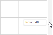
Scroll down to row 648, the first row of the Omega group listings. Notice the tiny ScreenTip near the scroll bar, for a live readout of the current row number as you drag the scroll box.
Select the entire row by clicking the 648 row heading number.
Click the Omega A worksheet tab at the bottom of the window.
Select row 2 by clicking the row heading number.
Hold the Shift+Ctrl keys and then press the Down Arrow key, which selects all the rows in the table.
Click the Copy button on the Home tab (or press Ctrl+C).
Click the Q1-2013 worksheet tab at the bottom of the window.
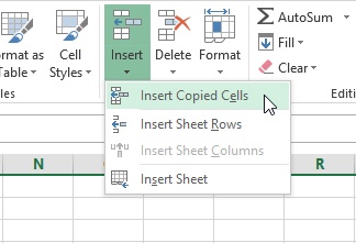
Click the arrow below the Insert button, located in the Cells group on the Home tab of the ribbon.
On the Insert menu, click Insert Copied Cells.
The new rows are inserted above the selected row. (Note that if you click the Insert button itself, rather than clicking the arrow button to display the Insert menu, Insert Copied Cells is still the default action.)
Click the Find & Select button in the Editing group on the Home tab, and then click Go To.
In the Reference box, enter E:E, and then press Enter.
You’ll notice that the entire column E is selected, just as if you had clicked the header. (You can use this same trick with rows; for example, entering 648:648 selects the entire row 648.)
With column E selected, click the Insert button arrow, and then click Insert Sheet Columns. (Again, pressing the button arrow and pressing the button itself both yield the same result.)
Select cell E1, enter Sale, and press Enter.
The next step is to add formulas to calculate totals. However, entering a formula into cell E2 and then dragging the fill handle to copy the formula down the column, with 1043 rows of data, is a lot of dragging. There’s an easier way.
With cell E2 still selected, click the Insert tab, and then click the Table button in the Tables group.
In the Create Table dialog box, click OK.
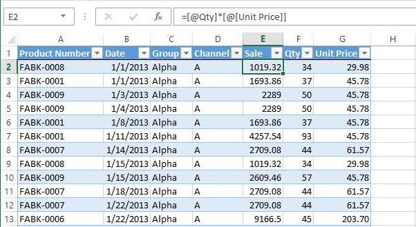
Select cell E2.
Enter = (an equal sign), and then press the Right Arrow key once.
Enter * (an asterisk), and then press the Right Arrow key twice.
Press Enter, and watch as Excel automatically fills the rest of the column with equivalent formulas.
The Excel table features made inserting these formulas very easy.
Tip
If youdon’t like the default table formatting, you can always choose another style. For example, you can switch back to the plain worksheet style used at the beginning of the exercise, by clicking the Table Tools Design tab (only available when the active cell is inside a table) and clicking the very first style in the Table Styles palette. You could also convert the table back to a regular cell range by clicking the Convert To Range button on the Table Tools Design tab. When you do so, the formulas are preserved, but they are converted from table reference formulas to regular Excel formulas.

Believe it or not, inserted cells are among the most common worksheet problems. When you insert text in Word, for example, existing text shifts to accommodate it, because text processing is essentially linear.
Spreadsheets (and tables in Word) are modular. When you insert cells, you force existing cells, rows, or columns to move out of the way. Unlike with text insertion, you have options when inserting cells: you can push existing cells either to the right or down. Inserting rows and columns is fairly safe, because this usually keeps related data aligned properly. But inserting cells can easily misalign data.
In this exercise, you’ll use the right approach to inserting and deleting cells, and you’ll discover what happens when you do it the wrong way.
Set Up
You need the FabrikamQ1-B_start.xlsx workbook located in the Chapter22 practice file folder to complete this exercise. Open the FabrikamQ1-B_start.xlsx workbook, save it as FabrikamQ1-B.xlsx, and then follow the steps.
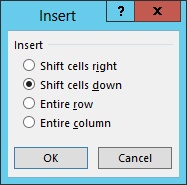
With the FabrikamQ1-B.xlsx workbook open, the Omega A tab active, and cell B2 selected, click the arrow below the Insert button in the Cells group on the Home tab, and then click the Insert Cells command to display the Insert dialog box.
Make sure the Shift cells down option is selected. (Even though the Entire row option would be the appropriate choice in this case, leave the default option selected.)
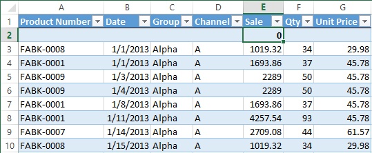
Click OK. Notice that all the other cells in the same column have been pushed down, and in the process, all the data in column B is now misaligned with all the other data in the table.
Scroll down to row 41, and notice that all the data in the column is now one cell lower, and all the sales records are now adjacent to incorrect dates.
Press Ctrl+Z to undo.
Click the Q1-2013 worksheet tab at the bottom of the screen; the worksheet contains an Excel table, and cell E2 is selected.
Click the arrow below the Insert button in the Cells group on the Home tab, click Insert Cells, and then click OK; this time Excel inserted an entire row in the table instead of a single cell (and duplicated the Sale formula automatically), demonstrating how Excel’s table features help ensure the integrity of your data.
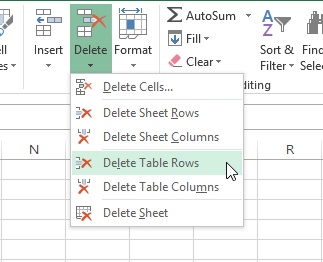
Click the arrow below the Delete button in the Cells group on the Home tab, and notice that, when a table is selected, two additional commands appear for table rows and table columns. (The equivalent commands also appear on the Insert menu.)
Click Delete Table Rows, which allows you to easily make modifications while leaving adjacent data on the worksheet undisturbed. Doing so removes only the selected rows in the table (in contrast, the Delete Sheet Rows command would remove selected rows all the way across the worksheet). Keep in mind, however, that inserting or deleting table rows or columns will still shift, and possibly misalign, adjacent cells.
Tip
Consider the possibility of future modifications when building worksheets. If you’d like to put more than one table of data on a single worksheet, inserting and deleting rows in one table could affect tables to the right, and inserting and deleting columns could affect tables following it. Instead, consider putting additional tables on separate sheets in the same workbook. For more information, see Creating a multisheet workbook later in this chapter.
Click the Seven-Year Financial Summary worksheet tab at the bottom of the screen.
Select row 8 by clicking its heading number.
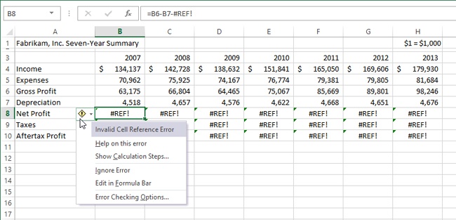
Click the Delete button on the Home tab, and notice the small triangles that now appear in the upper-left corner of each cell in rows 8 through 10, indicating that there is a problem with the formulas in those cells.
Click cell B8, and then click the action menu that appears adjacent to the cell.
There is not much the menu can offer that will help this time, other than Edit in Formula Bar, but there are a lot of cells to edit.
Press the Esc key to dismiss the menu.
Press Ctrl+Z to undo the last action and restore the deleted cells.
This is just a reminder that deleting cells can have consequences. In a large spreadsheet, you might not even be able to tell that something is wrong.

When you hear the words page layout, you probably think of printing, which used to be one of the top five issues reported by y product support. For Excel in 2013, printing has slipped down the list of issues considerably, perhaps because printing is easier than it used to be, or maybe because more people share data electronically or embedded in other documents like Microsoft PowerPoint presentations.
Of course, page layout is not just about printing, and especially in Excel, layout settings can actually affect not just printability, but the usability of a large worksheet.
In this exercise, you’ll work with panes, hidden columns, margins, and the print area.
Set Up
You need the UnitSales_start.xlsx workbook located in the Chapter22 practice file folder to complete this exercise. Open the UnitSales_start.xlsx workbook, save it as UnitSales.xlsx, and then follow the steps.
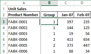
In the UnitSales.xlsx workbook, select cell B3.
Click the View tab.
Click the Split button in the Window group, and observe that Excel divides the worksheet into four segments, or panes, divided by gray bars. Each pane is more or less independent; the panes at the top will remain in place as you scroll down, and the panes at the left will stay in place as you scroll to the right. The Split button is a toggle; click it again to remove the split. If you needed only a single horizontal or vertical split, you could click and drag either gray bar off of the worksheet to remove it.
Making sure that cell B3 is still selected (and that the panes are still split), click the Freeze Panes button, and then click the Freeze Panes command in the menu that appears; the gray bars turn into thinner gray lines. Now the panes are locked; you can only scroll the lower-right pane. Rows 1 and 2 and column A all remain in place, which enables you to locate where you are in the worksheet at all times.
Scroll to the right and down.
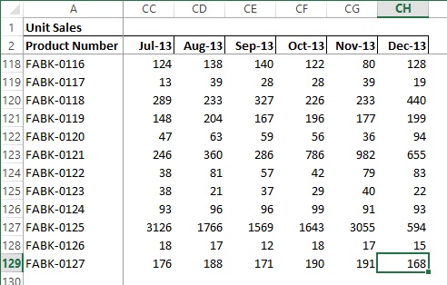
You can now navigate anywhere you want on the worksheet, and you’ll always be able to view the row and column headers. The following graphic illustrates this. Both cells A1 and CH129 are visible together onscreen.
Press Ctrl+Home to return to the upper-left corner of the worksheet. Notice that, with Freeze Panes active, the upper-left cell in the active pane (B3) is selected rather than A1, which is normally the case.
Click the column letter C to select the entire column.
Scroll to the right until column BV (labeled Dec-12) is visible.
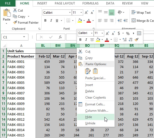
Hold down the Shift key and click the column letter BV to select all the columns except the 2013 totals.
Click the right mouse button anywhere in the selected column headers.
Click the Hide command to remove the selected columns from view, leaving only the 2013 columns visible.
(The Hide command can also be found on the Format menu’s Hide and Unhide submenu.) The relevant data on the worksheet is now easier to use, and the sheet is much easier to navigate. But you might want to print it, too.
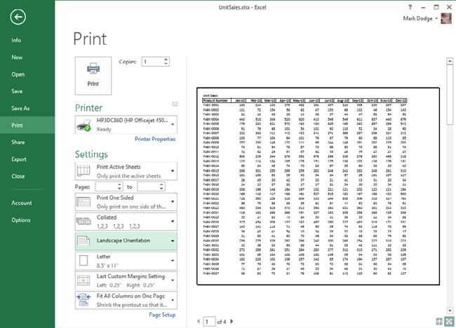
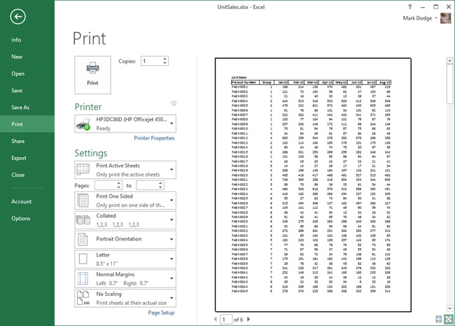
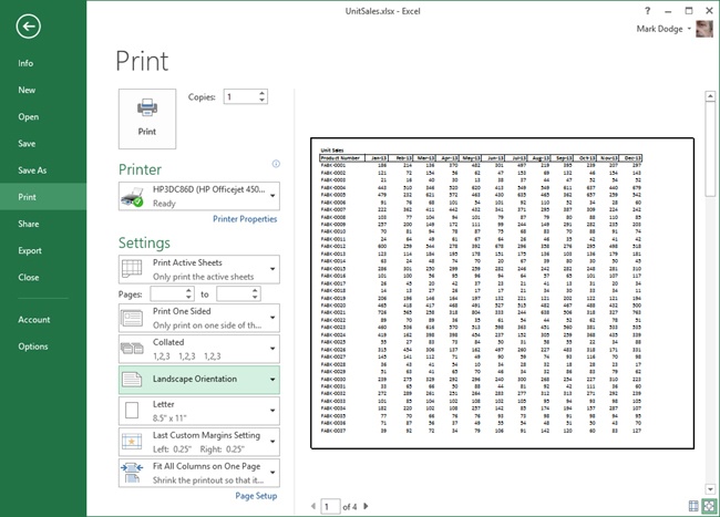
Click the File menu, and then click Print to display the Print Preview window. Look at the preview image; not all the columns are visible; look at the bottom of the screen and notice that it will take six pages to print this sheet.
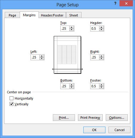
Click the Margins button (which currently displays Normal Margins), and then click Custom Margins to display the Page Setup dialog box.
Double-click each number in the Top, Bottom, Left, and Right boxes, and change them all to .25. Then select Vertically for the Center on page option. (Headers and footers are not used in this exercise, so don’t worry about changing those numbers. Headers and footers wouldn’t fit with such narrow margins, anyway.)
Click OK.
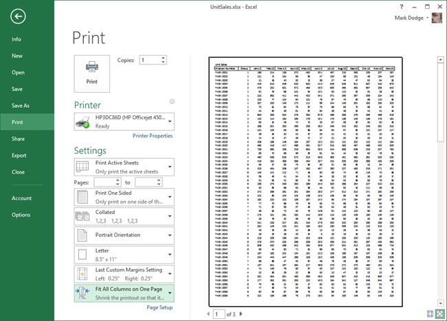
Click the Scaling button (which is currently set to No Scaling) and click Fit All Columns on One Page; notice that now, January through December are visible in the preview, and that this sheet will now require only three pages to print.
Press the Esc key to close the Print Preview window. These and any other print and page layout settings you make are preserved the next time you save, so that the sheet will print the same way the next time you open it.
Press Ctrl+Home to return to cell B3.
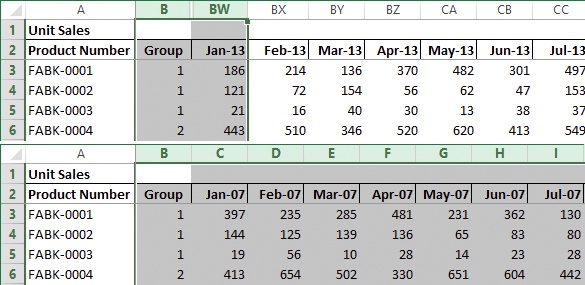
Drag through the B and BW column headers to select them.
On a selected column header, click the right mouse button, and then select the Unhide command.
Click the View tab, and then click the Split button to turn off the split/frozen panes.
Press Ctrl+Home and notice that this time, with panes unfrozen, cell A1 is selected.
Press Ctrl+G to display the Go To dialog box.
Enter Z119 in the Reference box.
Hold down the Shift key and click OK to select the range A1:Z119.
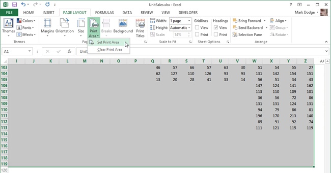
Click the Page Layout tab, click the Print Area button, and then click Set Print Area.
Click the File tab and click Print to display the Print Preview screen; notice that the sheet is still set up to include all the columns on one page.
Click the Orientation button (which currently shows Portrait), and then click Landscape.

The Print Titles command, located on the Page Layout tab, allows you to specify rows and columns—typically containing labels identifying your detail data—to print on every page. This is similar to freezing panes, except that it only applies to printing, and you can specify any cell range on the worksheet, whether or not it happens to be adjacent to the labels.
In the previous exercise, you used the Hide command to conceal data that you didn’t need to either display or print. In this exercise, you’ll define the print area and print titles to customize your printed work.
Set Up
You need either the UnitSales.xlsx workbook from the previous exercise or the UnitSales_start.xlsx workbook located in the Chapter22 practice file folder to complete this exercise. If you are using the UnitSales_start.xlsx workbook, open it and save it as UnitSales.xlsx. Then follow the steps.
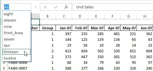
Open the UnitSales.xlsx workbook, if it is not already open.
Click the Name box at the left end of the formula bar, and select the named range thirteen.
Click the Page Layout tab.
Click the Print Area button, and then click Set Print Area.
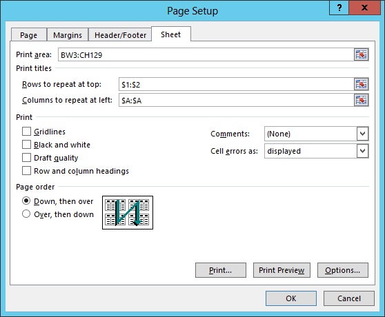
Click the Print Titles button in the Page Setup group on the Page Layout tab to display the Page Setup dialog box with the Sheet tab active.
Notice that the Print Area box already displays the reference BW3:CH129, the definition of the named range thirteen.
Click in the Rows to repeat at top box and then, on the worksheet, drag through row headings 1 and 2 to select the entire rows.
Notice that when you click the worksheet, the dialog box collapses, revealing any cells that were hidden beneath. (You may need to scroll up a bit to view rows 1 and 2.) This type of box enables you to navigate around the worksheet, and then select cells, rows, or columns, which serves to enter their references into the box.
Click in the Columns to repeat at left box, and then click the column A heading to select it. (Again, scroll to the left if necessary to make column A visible.)
Click the Print Preview button in the Page Setup dialog box.
Click the Orientation button (which usually displays Portrait Orientation), and select Landscape Orientation.
Using the Print Titles command enables you to specify any range on the worksheet that you want to print, and includes the appropriate titles for you. This setting is saved with the worksheet. If you want to print another range, all you need to do is specify a different print area; you won’t need to change the print titles again unless you add more rows or columns of information that you want to include.
When you’re printing large Excel worksheets, the location of page breaks can be a real problem. If your table is a little bit too wide to fit on a sheet, for example, you may need to print a second page containing a single column, doubling the necessary size of the printout (for example, 10 pages become 20). Excel provides some help with this.
In this exercise, you’ll control page breaks and page size by using Page Break Preview.
Set Up
You need either the UnitSales.xlsx workbook from the previous exercise or the UnitSales2_start.xlsx workbook located in the Chapter22 practice file folder to complete this exercise. If you are using the UnitSales2_start.xlsx workbook, open it and save it as UnitSales.xlsx. Then follow the steps.
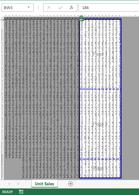
In the UnitSales.xlsx workbook, click the Name box at the left end of the formula bar and enter the cell address BW3.
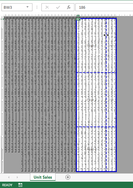
Click the View tab, and then click the Page Break Preview button.
This workbook already has a defined print area (as shown in the previous exercise): the white area visible in Page Break Preview mode. Each printed page has a watermark number superimposed on it in this view. Don’t worry, the numbers won’t print.
Click the Zoom button, in the Zoom group, on the View tab.
In the Custom box, enter 20, and press Enter. (Your screen size may differ, so feel free to scroll and adjust your zoom so that all of the white areas of the worksheet are visible in Page Break Preview.)
Click the Page Layout tab.
Click the Orientation button, and then click Portrait; the display adjusts and shows that you will now print six pages; the dotted blue lines indicate page breaks. You can drag the blue lines around in Page Break Preview mode. Page breaks will adjust accordingly, and the worksheet will be scaled to accommodate, if necessary.
Point to the vertical dotted line until the pointer turns into a double-headed arrow.
Click the vertical dotted blue line and drag it to the right, past the solid blue line. Take a look at the Scale percentage in the Scale to Fit area of the Page Layout tab; after you dragged the line, it changed to the percentage necessary to squeeze all the columns across one page for printing.
Click the View tab, and then click the Normal button to cancel Page Break Preview mode.
Press Ctrl+Home to display cell A1.
Tip
Many View tab settings are saved with the workbook, including Page Break Preview. When you open a workbook, these settings as well as the active cell (or cell range) that was selected when you last saved are visible onscreen. You might want to change the view and select cell A1 or another cell in the main area of the worksheet before saving, especially if you share the workbook with others. In a multisheet workbook, the active sheet is also saved.


Workbooks can contain as many worksheets as you can create, limited only by your good sense and your computer’s memory. Putting multiple tables, data sets, presentation graphics, and similar items on a single sheet is not only unnecessary, it’s probably unwise, as tempting as it may be to leverage a million rows and 16 thousand columns of sheet real estate. You can help maintain the integrity of your data and make it easier to work with by breaking free of the single-worksheet mindset. (For some good reasons not to put more than one table on a sheet, see Inserting and deleting cells, earlier in this chapter.)
In this exercise, you’ll create a multisheet workbook, format the sheets together, and then use selection and copying techniques to move data into them.
Set Up
You need the Q1-Transactions_start.xlsx workbook located in the Chapter22 practice file folder to complete this exercise. Open the Q1-Transactions_start.xlsx workbook, save it as Q1-Transactions.xlsx, and the follow the steps.
In the Q1-Transactions.xlsx workbook, click the New Sheet button twice (the plus-sign button next to the sheet tab at the bottom of the worksheet window) to add two new sheets to the workbook.
Double-click the Q1-2013 tab, so that the name of the tab is highlighted.
Enter Jan 2013 and press Enter.
Double-click the Sheet1 tab, enter Feb 2013, and press Enter.
Double-click the Sheet2 tab, enter Mar 2013, and press Enter.
Click the Jan 2013 sheet tab.
Select cells A1:F1 (the column labels).
Press Shift, and then click the Mar 2013 sheet tab to select all three sheets. Notice that [Group] now appears after the file name at the top of the Excel window.
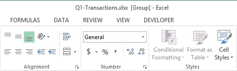
Click the Home tab on the ribbon.
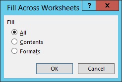
Click the Fill button in the Editing group, and then click Across Worksheets, a command that only appears when you have multiple worksheets selected.
Make sure that All is selected in the Fill Across Worksheets dialog box, and then click OK. After this, you need to make sure that only one worksheet is selected, otherwise all the edits you make to the active sheet will be performed on the other selected sheets as well.
Click the Feb 2013 sheet tab (which serves to deselect the group of sheets), then click the Jan 2013 tab again.
Select cell B2 (the first date in the Date column).
Click the Data tab on the ribbon.
Click the Sort A to Z button in the Sort & Filter group; the button is now labeled Sort Oldest to Newest because the currently selected cell contains a date value.
Press Ctrl+F to display the Find and Replace dialog box.
Enter 3/1/2013 into the Find What box and press Enter.
Click the Close button or press Esc to close the dialog box.
Press the Left Arrow key to select the cell in column A adjacent to the date.
Hold down the Shift and Ctrl keys, and then press the Right Arrow Key to select all the data in the row.
Press the Shift and Ctrl keys, and then press the Down Arrow key to select all the rows of the table below, containing March transactions.
Press Ctrl+X to cut the selected cells.
Click the Mar 2013 sheet tab.
Select cell A2, and then press Ctrl+V to paste the cut cells.
Click the Jan 2013 sheet tab, and then click any cell to deselect the empty range where you just removed cells. (If you don’t do this, the next step won’t work, because Find searches only the selected cells if more than one is selected.)
Press Ctrl+F, enter 2/1/2013, and press Enter.
Close the dialog box, and then press the Left Arrow key to select the adjacent cell in column A.
Hold down the Shift and Ctrl keys, and then press the Right Arrow key to select the row of data.
Press the Shift and Ctrl keys, and then press the Down Arrow key to select all the February transactions.
Press Ctrl+X to cut the selected cells.
Click the Feb 2013 sheet tab.
Select cell A2, and then press Ctrl+V to paste the cut cells.


After you add sheets to a workbook, you can change their order; insert, delete, move, or copy sheets to other workbooks; or even create new workbooks from sheets.
In this exercise, you’ll move, rename, and copy sheets in a workbook, and drag sheets between workbooks.
Set Up
You need either the Q1-Transactions.xlsx workbook from the previous exercise or the Q1-Transactions2_start.xlsx workbook located in the Chapter22 practice file folder to complete this exercise. If you are using the Q1-Transactions2_start.xlsx workbook, open it and save it as Q1-Transactions.xlsx. Then follow the steps.
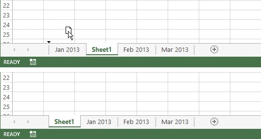
In the Q1-Transactions.xlsx workbook, click the Add Sheet button (the plus sign) next to the sheet tabs at the bottom of the workbook window. Sheet1 appears between the Jan 2013 and Feb 2013 tabs.
Click the Sheet1 tab and drag it until the black arrow indicator is to the left of the Jan 2013 tab.
Double-click the Sheet1 tab, enter Summary, and press Enter.
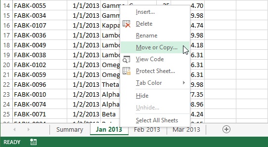
Right-click the Jan 2013 tab to display the shortcut menu.
Tip
Hiding a worksheet may be desirable if it contains information that others don’t need to view but that may be vulnerable or unnecessarily confusing (such as formulas used to calculate values used elsewhere, or critical reference data that never changes). Hide the current worksheet by clicking the Format button on the Home tab and selecting Hide Sheet on the Hide & Unhide menu, or by right-clicking the tab of the sheet you want to hide and then clicking Hide. Once a sheet is hidden, you can unhide it with the Unhide command, which appears in the same locations as the Hide command, but only if a hidden sheet is present.
Click the To Book list and select (new book).
Select the Create a copy check box.
Click OK, and Excel creates a new, unnamed workbook containing a copy of the Jan 2013 worksheet.
Click the View tab.
Click the Arrange All button, select Horizontal, and then click OK.
Click the Feb 2013 tab in the Q1-Transactions.xlsx workbook.
Hold down the Ctrl key and drag the Feb 2013 tab to the other workbook; you’ll notice that a small page icon with a plus sign in it appears next to the pointer, indicating a copy operation (if you didn’t hold down Ctrl, you would move the sheet rather than copy it, and no plus sign would appear in the icon).
Release the mouse button and the Ctrl key.


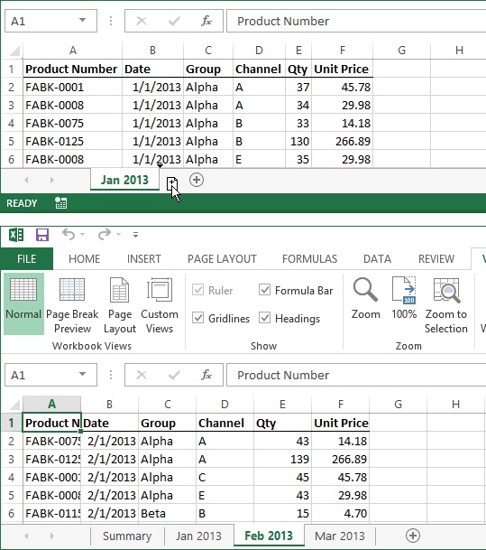
Now that you’ve created a multisheet workbook, you need to be able to work with the data on those sheets. The sample workbook used in the following exercise is similar to the Q1-Transactions workbook used in the previous exercise, but formatting was added on the Summary sheet, and a column of totals was added to each detail sheet by using the technique described in Inserting rows and columns, earlier in this chapter.
In this exercise, you’ll use a basic summary sheet to summarize important data by using formulas that calculate data located on the detail sheets.
Set Up
You need the Q1-Summary_start.xlsx workbook located in the Chapter22 practice file folder to complete this exercise. Open the Q1-Summary_start.xlsx workbook, save it as Q1-Summary.xlsx, and then follow the steps.
On the Summary sheet of the Q1-Summary.xlsx workbook, select cell C5.
Enter =SUMIFS(.
Click the Jan 2013 sheet tab, and then click the E column header to select the entire column.
Press F4 to change the reference to fixed ($E:$E).
Enter a comma.
Click the C column header to select the entire column.
Press F4 to change the reference to fixed ($C:$C).
Enter a comma.
Click the Summary sheet tab, click cell B5, and then press F4 three times to change the reference to mixed ($B5).
Press Enter.
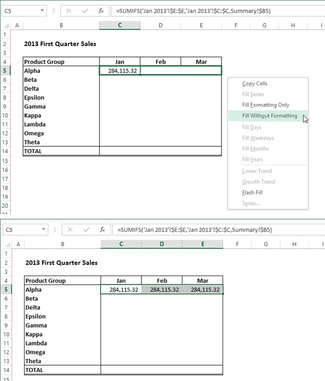
Select cell C5, right-click the fill handle in the lower-right corner of the cell, and drag to the right to cell E5; a menu appears.
Click Fill Without Formatting to copy the formula without disturbing the border formats.
Select cell D5, double-click the formula bar to enable Edit mode (indicated in the status bar at the lower-left corner of the window), and change Jan to Feb in both references (being careful not to disturb adjacent spaces and apostrophes when deleting and typing.)
Press Enter.
Select cell E5, double-click the formula bar, and change Jan to Mar in both references.
Press Enter.
Select cells C5:E5.
To copy the formulas to the rest of the table, right-click the fill handle in the lower-right corner of cell E5 and drag down to cell E13; a menu appears.
Click the Fill Without Formatting command to copy the formulas down the table without disturbing the border formats.
With all the formulas still selected, click the Decrease Decimal button in the Number group on the Home tab twice.
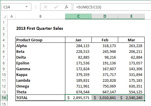
Select cells C14:E14.
Click the AutoSum button in the Editing group on the Home tab.
Let’s take a closer look at one of the monthly Product Group formulas created in the previous exercise. The SUMIF function simply allows you to use criteria to select specific values to add, all of which reside on other worksheets in the example. Each of the three sections of this formula contains a sheet reference, characterized by the presence of an exclamation point separating the sheet name from the cell address.
Formula |
| ||
Function and arguments |
| ||
|
|
| |
Sheet references |
|
|
|
Description | Refers to the totals in the Sale column on the Jan 2013 sheet | Refers to the totals in the Group column on the Jan 2013 sheet | Refers to the names in the Product Group column on the Summary sheet |
A cell reference such as $B5 used in a formula always refers to a cell on the same sheet. But if you precede a cell reference with a sheet reference, such as Summary!, you can access values on the Summary sheet from any sheet in the workbook.
Just one criterion was used in these formulas (the Product Group name), but you can add up to 127 criteria, each with its own criteria range. Notice the difference between the references for Criteria Range and Criteria. The Criteria Range sheet name is enclosed in single quotation marks (apostrophes, if you prefer), but the Criteria reference is not. If a reference includes a space character, as in the sheet name Jan 2013, you must enclose it in single quotation marks.
If you have a set of identical sheets in a workbook (unlike the Q1-Summary workbook), you can use a multisheet reference to summarize values located in the same cell on each sheet. These are sometimes called “3-D references,” since they escape the two-dimensional spreadsheet grid, drilling down into a stack of worksheets. For example, if a workbook contains a set of sales totals sheets for each month (named Jan, Feb, Mar, and so on) and cell B5 contains the equivalent value on each sheet, the following formula on the Summary sheet adds up the values in cell B5 on all the monthly sheets.
=SUM(Jan:Dec!B5)
The multi-sheet reference is similar to the sheet reference in the SUMIFS formula. Just take the names of the first and last sheets in the stack you want to summarize, and separate them with a colon to create a multisheet reference. And, of course, you need to surround the multisheet reference with single quotation marks if the sheet names include spaces.
=SUM('Jan 2013:Dec 2013'!B5)You can open as many workbooks at once as your computer’s memory allows, and you can move among them by pressing Alt+Tab, the system shortcut for switching windows. This is relatively new behavior in Excel. Earlier versions embraced all open workbooks under one umbrella, so to speak; a single “instance” of Excel. Now, each workbook you open generates a new window—another instance of Excel—each with its own ribbon, sheet tabs, status bar, and so on. You may appreciate this behavior if you use multiple monitors.
In the previous chapter, we explored opening additional windows to view other areas of the same workbook, or to simultaneously view the same area in different ways. (For more information about view options, see Setting view options in Chapter 21.) Windows that you create this way look nearly identical to windows of other open workbooks, because they both create separate instances of Excel. One way to tell the difference is by looking at the workbook name displayed at the top of the screen. It is a window on a workbook if the name includes a colon followed by a number (indicating which window you’re looking at, such as Book1.xlsx:5). Otherwise, the instance in question is a different workbook.
In this exercise, you’ll create another workbook window and arrange workbooks and windows together on the screen.
Set Up
You need both the UnitSales_start.xlsx and FabrikamQ1_start.xlsx workbooks located in the Chapter22 practice file folder to complete this exercise. Open the UnitSales_start.xlsx workbook, and save it as UnitSales.xlsx. Open the FabrikamQ1_start.xlsx workbook, and save it as FabrikamQ1.xlsx. Then follow the steps.
Activate the UnitSales.xlsx workbook.
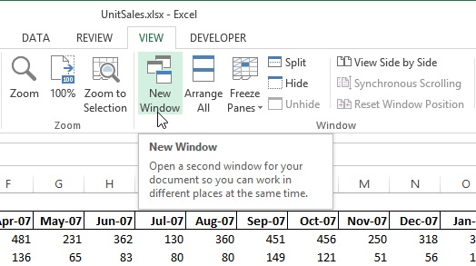
Click the View tab, and then click New Window.
Notice that the workbook name displayed in the title bar becomes UnitSales.xlsx:2.
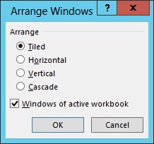
Click the Arrange All button in the Window group on the View tab, and then select the Windows of active workbook check box.
Click OK, and you’ll notice that both active workbook windows are displayed side by side, ignoring the other open workbook. The title bars of the windows display the names UnitSales.xlsx:1 and UnitSales.xlsx:2.
On the View menu of the UnitSales.xlsx:2 window, click the View Side by Side button.
In the Compare Side by Side dialog box, select UnitSales.xlsx:1 and click OK; the windows rearrange to horizontal tiling orientation. Notice that in the Windows group on the View tab, the Synchronous Scrolling button is highlighted automatically when you click the View Side by Side button.
Scroll up and down in the active window; the inactive window scrolls along with it.
Click the View Side by Side button again to turn it off; the windows rearrange to vertical tiling.
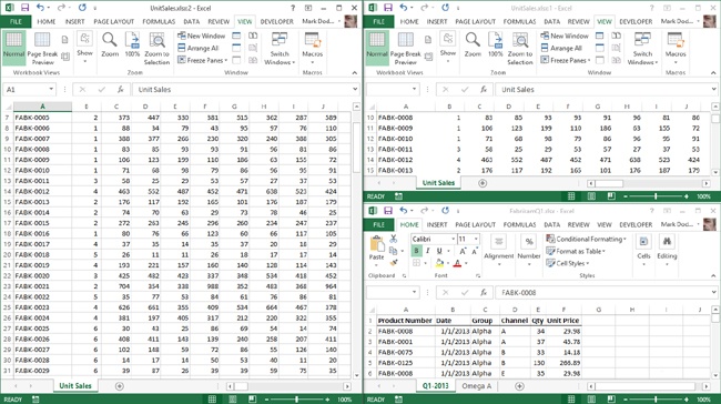
Click the Arrange All button again, select Tiled, and make sure that the Windows of active workbook check box is cleared.
Click OK, and another window appears, displaying the FabrikamQ1.xlsx workbook (as well any other workbooks that you may have open).
Click the UnitSales.xlsx:1 window to activate it.
On the View tab, click the Hide Window button in the Window group, and the window disappears from the screen. Notice, however, that the remaining window still displays UnitSales.xlsx:2 in its title bar.
Click the Save button at the top of the Unit Sales window.
Click the close window button (the X) in the upper-right corner of the Unit Sales window.
Click the File tab, click the Open command, and select the Unit Sales workbook you just closed (which should be near the top of the Recent Workbooks list). Notice that nothing seems to happen. Because the main window was hidden when you saved the Unit Sales workbook, it is open, but not visible.
On the View tab, click Unhide, which is only available if a hidden window is present. The UnitSales.xlsx filename is highlighted in the dialog box.
Click OK to unhide the workbook.
Click the Save button to save the workbook without the hidden window.
Excel’s table features make it easier and safer to insert and delete rows and columns, as well as add rows or columns of formulas.
You can convert tables back to regular cells by using the Convert To Range command.
Use the Print Titles command to specify row and column labels to be printed on each page.
Use the Freeze Panes command to keep row and column labels in view on screen.
Page Break Preview allows you to adjust page breaks by dragging.
To keep track of related data in the same workbook, click the New Sheet button to create additional sheets.
You can summarize data in a multisheet workbook with formulas, by using sheet references.
You can arrange all open workbooks and windows together on your screen by using the Arrange All button.