Chapter 5

The Random Waypoint Model

We have seen in the previous chapter that a major shortcoming of random walk models is the lack of a fundamental aspect of intentional mobility, namely, the notion of trajectory of a movement. Indeed, random walks are aimed at mimicking completely random movement patterns, and as such they can be considered as relatively accurate in describing mobility patterns where mobile entities display such highly random behavior.

Are there many next generation wireless network application scenarios where node mobility can be classified as “highly random?” Unfortunately (or luckily, depending on the viewpoint), the answer is no: apart from a few wireless sensor network scenarios (e.g., animal tracking in open environments, in which mobility can be faithfully modeled by Lévy flights), in the vast majority of next generation wireless network scenarios node mobility is not random, but obeys some (often strict) rules.

The random waypoint model (RWP), first defined by Johnson and Maltz (1996) to study the performance of a routing protocol for MANETs, can be considered as a first attempt to define a simple, synthetic mobility model aimed at modeling intentional human movement. Thus, from the viewpoint of modeling accuracy, and despite its several shortcomings as described in this chapter, the RWP model can be considered a breakthrough in next generation wireless network mobility modeling compared to random walks. This, combined with the popularity of the Dynamic Source Routing (DSR) protocol for MANETs introduced in Johnson and Maltz (1996), now part of the IEEE 802.11 standard, explains the success of this mobility model. The RWP model is in fact by far the most widely used mobility model in next generation wireless network simulation, and it is provided as a default mobility model in popular wireless network simulators such as Ns2 (Ns2Team 2011), GloMoSim (Team 2011a), GTNetS (Team 2011b), etc.

The popularity of the RWP model has partly declined recently, mainly due to some research work highlighting possible inaccuracy in simulation results that might occur if the RWP model is not used properly; one of the case studies in Part Seven of this book will be devoted to this topic. Another factor negatively impacting RWP model popularity is the “specialization” trend observed in next generation wireless network research in recent years: as commented in Section 1.2, the concept of “general-purpose” MANET for which the RWP model was originally defined is being replaced by narrower scoped network architectures and scenarios such as vehicular networks, opportunistic networks, and so on. Thus, mobility models specifically defined for the scenario at hand, like the ones presented later in this book, have gained popularity in recent years.

Considering its past and present popularity, the RWP mobility model is by far the most thoroughly studied mobility model for next generation wireless networks, and several of its fundamental properties have been characterized in the literature. In this chapter, after a formal definition of the RWP mobility model, we will present a characterization of the two most important properties of RWP mobile networks, namely, the stationary node spatial distribution and average nodal speed. For both these properties, we will report not only the characterization, but also some details about their derivation. This should show the reader how significant examples of tools from geometric probability and statistics are used within the field of mobility modeling. We will then conclude by presenting variations of the basic RWP model which have been proposed.

5.1 The RWP Model

Similar to random walk models, the RWP model belongs to the class of synthetic, entity-based mobility models. In particular, this means that the mobility of different network nodes is modeled by independent stochastic processes. Hence, a mobile network with n nodes is modeled by means of n replicas of the same stochastic process governing the mobility of a single node. In the following, we describe such a stochastic process.

Informally speaking, the RWP mobility model in a d-dimensional spatial domain R is defined by initially selecting the position of the node uniformly at random in R. After a predefined pause time t_p, a parameter of the model, the node selects a destination—called waypoint—uniformly at random in R, and starts moving along a straight-line trajectory toward the waypoint with constant speed v chosen uniformly at random in an interval [v_min, v_max], where v_min and v_max are two further parameters of the model. Once the waypoint is reached, the node pauses at the waypoint for time t_p. Then, it starts a new trip according to the same rules: the next waypoint is chosen uniformly at random in R; the node moves along a straight-line trajectory toward the waypoint with random speed, etc.

More formally, a RWP mobile node is defined by the following stochastic process:

where D_i is a d-dimensional random variable corresponding to the coordinates of the ith waypoint, T_i is the pause time at the ith waypoint, and V_i is a random variable corresponding to the node speed during the trip toward the ith waypoint. In the original RWP definition, D_i is uniformly distributed on R, T_i is a constant equal to t_p, and V_i is chosen uniformly at random in [v_min, v_max]. The position of the initial node position D₀ is also selected uniformly at random in R.

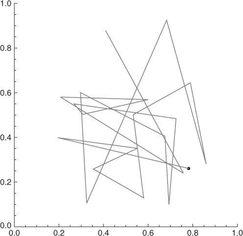
An example of RWP mobility in the unit square R = [0, 1]² is shown in Figure 5.1: the starting point is the black dot; the next waypoint is chosen uniformly at random in R, with the node moving along a linear trajectory. The figure reports the trajectory followed by the node during 20 mobility steps.

Figure 5.1 An example of two-dimensional RWP mobility in the unit square.

Two observations about RWP mobility are in order:

5.2 The Node Spatial Distribution of the RWP Model

The stationary node spatial distribution is the first fundamental property of RWP mobility to have been investigated in the literature. The above-described border effect was first noticed and quantitatively measured in some simulation-based studies (e.g., Bettstetter and Krause (2001), Blough et al. (2002)); then, the border effect was formally characterized through derivation of the stationary node spatial distribution.

Before proceeding further, the reader might question why characterizing the stationary node spatial distribution of a mobility model is considered a very important problem within the wireless networking research community. The answer to this question lies in the fact that a stationary node spatial distribution which is different from the initial distribution of nodes (which is typically random uniform) can severely impair simulation accuracy. The impact of the RWP stationary node spatial distribution on simulation accuracy will be discussed extensively in Part Seven of this book.

The stationary node spatial distribution of a RWP mobile node moving in the unit square was first closely approximated by Bettstetter et al. (2003). Later on, Hyytia et al. (2006) derived the exact node spatial distribution for arbitrary convex two-dimensional shapes of the spatial domain R and for arbitrary waypoint distribution. In this section, we present their approximate derivation, which is more intuitive. In what follows, the spatial domain is assumed to be the unit square R = [0, 1]².

Consider a RWP mobile node defined by the stochastic process {D_i, t_p, V_i} as defined in the previous section, and let d_i = (x_i, y_i) denote the ith realization of random variable D_i. A first important result proven by Bettstetter et al. (2003) concerns the mean ergodicity of the sequence of random variables {L_i}, where , that is, the sequence of random trajectory lengths. Ergodicity is one of the most important notions in statistics, and states that a stochastic process {X₁, X₂, …} is ergodic when, for large enough k, taking k samples from a single random variable (e.g., X₁) is statistically equivalent to taking a single sample from k of the X_i variables. Thus, the mean ergodicity result stated by Bettstetter et al. (2003) implies that the mean of a set of samples taken from random variables {L₁, L₂, …} (one sample for each random variable) is the same as that obtained by repeatedly sampling from a single random variable, say L₁. Note that this result is not immediate, since random variables L_i and L_i+1 are not independent: in fact, two consecutive trajectories share an endpoint. However, random variables L_i and L_i+2 are indeed independent, since they do not share endpoints. Sequence {L_i} can then be divided into two sub-sequences {L_2k} and {L_2k+1} of even and odd trips, respectively, with the property that mean ergodicity holds for both sub-sequences. Due to linearity of the mean, the mean ergodicity of the entire sequence {L_i} then follows.

Why is the mean ergodicity result so important? To understand this result, let us start by investigating the effect of the pause time on the node spatial distribution. Let us consider the position (x_t, y_t) of a mobile node u at time t, for a sufficiently large t. According to the RWP model definition, node u can be in one of two possible states at any instant of time: pausing, if it is resting at a waypoint; or traveling, if it is traveling toward the next waypoint. Let S_t denote the random state of node u at time t, with S_t taking values P (pause) or T (travel). The node spatial distribution of the RWP model, that is, the pdf of (x_t, y_t) as t → ∞, can be defined as follows:

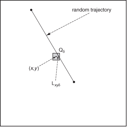
where f_P(x, y) = U(x, y) is the pdf of waypoints (i.e., the uniform distribution in R), f_T(x, y) is the pdf of a node when traveling between consecutive waypoints, and Prob(S = P) = lim_t→∞Prob(S_t = P) (respectively, Prob(S = T)) is the stationary probability of finding the node in state P (respectively, T). Thus, in order to obtain f_RWP, we need to derive the node spatial distribution f_T of a node moving along a trajectory whose endpoints are chosen uniformly at random in R, which is called the mobility component of the distribution. The mean ergodicity property implies that this problem is equivalent to that of computing the intersection between a segment with uniformly chosen endpoints and a small area, say, a square of side δ with 0 < δ 1 centered at a certain position (x, y). The latter problem can then be solved using tools from geometrical probability.

Figure 5.2 depicts the situation. The goal is to compute the probability mass lying in a small square Q_δ of side δ > 0 centered at an arbitrary position (x, y) ∈ R, that is, the probability P_t(x, y, δ) of finding node u in Q_δ at time t, for t → ∞. We first observe that, if δ is sufficiently small, the pdf f_T can be considered to be constant in Q_δ. Thus, we can write

and

where P(x, y, δ) = lim_t→∞P_t(x, y, δ).

Figure 5.2 The derivation of the mobility component of distribution f_RWP.

We are then left with the business of evaluating P(x, y, δ). To this end, we first observe that in the RWP model, node velocity during a specific trip, although randomly selected at the beginning of the trip, is constant; thus, taking any trajectory in the sequence of trips {D_i, t_p, V_i}, and taking two equal length portions (segments) s₁, s₂ within this trajectory, we have that the amount of time that the node spends in s₁ is the same as that spent in s₂. This implies that space and time are equivalent quantities in the RWP model, and P(x, y, δ) can be expressed as the ratio between the expected length of the intersection L_xyδ of a random trajectory with square Q_δ and the expected length of a random trajectory. In other words, we can write

Quantity E[L] represents the expected length of a random segment with uniform endpoints in the unit square, which is known from the geometric probability literature to be equal to 0.521 405 (Santaló 2002).

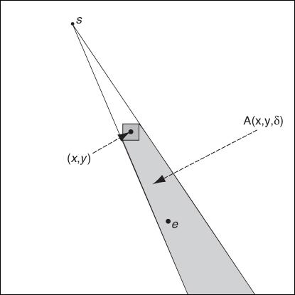
Deriving E[L_xyδ] is more complicated. Let us fix the position d_i−1 = s of the trajectory starting point (waypoint i − 1). It can immediate be seen that L_xyδ ≠ ∅ if and only if the endpoint of the trajectory (waypoint d_i = e) lies within a subregion of R, represented as the shaded area in Figure 5.3 and denoted A(x, y, δ). Under the simplifying assumption that the length l_xyδ of segment L_xyδ is expressed as (here it comes as the approximation in Bettstetter et al.'s approach)

Figure 5.3 Derivation of E[L_xyδ].

we can write

where the notation A(x, y, δ) in the right hand side integral above is slightly abused to denote the area of the corresponding region.

The integral on the right hand side of the formula at the end of the previous page can be exactly computed by properly partitioning R based on the shape of the A(x, y, δ) regions. The derivation is quite lengthy and is not reported here—the interested reader is referred to Bettstetter et al. (2003). The resulting expression for f_T in the region (0 ≤ x ≤ 0.5) ∪ (0 ≤ y ≤ x)—values of f_T in the other regions of R are obtained by symmetry—is

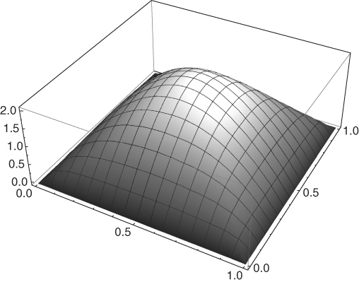
Density function f_T is shown in Figure 5.4. As can be seen in the figure, the mobility component of the RWP model spatial density function is bell-shaped, with a relatively higher node density in the center of the spatial domain R.

Figure 5.4 The mobility component of the RWP model spatial density function.

The last step in the derivation of the RWP model node spatial distribution is to compute probabilities Prob(S = P) and Prob(S = T). These probabilities, under the assumption that node speed is kept constant at v > 0 (i.e., v_min = v_max = v > 0), can be easily computed as follows:

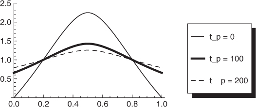
The resulting distribution f_RWP when t_p = 50 and v = 0.01 (corresponding to 10 m/s if the unit side is considered to be 1 km) is displayed in Figure 5.5. It is interesting to observe that, in accordance with intuition, a relatively longer pause time results in a relatively flatter (i.e., more uniform) node spatial distribution. This is shown in Figure 5.6, which displays the diagonal cross-section of the distribution for different values of pause time.

Figure 5.5 The RWP node spatial distribution with t_p = 50 and v = 0.01.

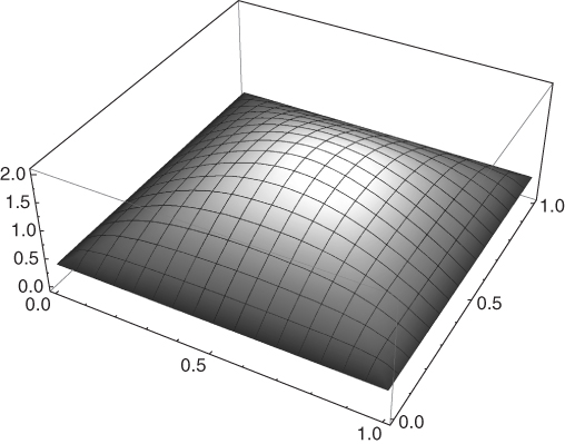
Figure 5.6 Diagonal cross-section of the RWP node spatial distribution with v = 0.01 and different values of pause time t_p.

5.3 The Average Nodal Speed of the RWP Model

A second property of the RWP model that has been studied in the literature is the stationary average nodal speed, which is formally defined as follows.

Assume that n nodes move independently within a spatial domain R according to the RWP mobility model, and denote by v_i(t) the instantaneous speed of the ith node at time t. The stationary average nodal speed v_RWP is defined as

Similar to the stationary node spatial distribution, interest in the stationary average nodal speed lies in the fact that its characterization allows correct setting of the simulation parameters, as we will see in Part Seven of this book.

The stationary average nodal speed of the RWP model was first studied by Yoon et al. (2003), who evaluated the stationary average nodal speed through simulation, and formally derived the value of v_RWP.

The value of v_RWP was derived under the following assumptions:

While the second and third assumptions are indeed part of the RWP model definition, the first assumption apparently changes considerably the features of RWP mobility. However, Yoon et al. (2003) prove that assumption 1 above, which is made to simplify the analysis, has no effect on the value of v_RWP.

To derive v_RWP, Yoon et al. describe the RWP mobility model as a stochastic process {V_i, D_i, S_i}, where V_i is the random variable denoting the velocity during trip i, D_i is the random variable denoting distance traveled during trip i, and S_i is the random variable denoting travel time during trip i. Setting , then v_RWP can be expressed as follows:

where K(T) is the total number of trips undertaken within time T, including the (possibly incomplete) last one, and d_k (resp., s_k) is the travel distance (resp., time) of trip k.

Thus, similar to the derivation of the stationary node spatial distribution, the computation of v_RWP is reduced to the problem of computing the ratio of the expectations of two random variables, namely D_i and S_i. Yoon et al. (2003) show that

yielding

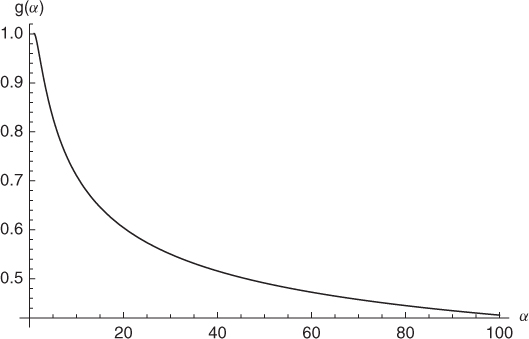
What are the implications of the above characterization of v_RWP? A first important observation is that v_RWP is at most as large as the initial average nodal speed v₀ = (v_min + v_max)/2. To see why this inequality holds, it is sufficient to study the following function:

where α = v_max/v_min > 1. The behavior of g(α) for increasing values of α > 1 is displayed in Figure 5.7. As can be seen from the plot, g(α) is always below 1, implying that the stationary average nodal speed is at most as large as the initial speed v₀. This phenomenon is known as the speed decay phenomenon, and Yoon et al. (2003) also observed it experimentally. Furthermore, lim_α→∞g(α) = 0, implying that when the maximal velocity v_max becomes asymptotically larger than the minimal velocity v_min, the stationary average nodal speed becomes asymptotically smaller than the initial speed. Thus, in this case the speed characteristics are substantially different between the beginning and steady state of the mobility process.

Figure 5.7 Behavior of function g(α) for increasing values of the ratio α between maximal and minimal node speed.

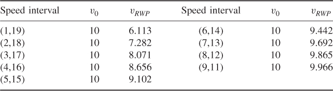
Another interesting observation is that , that is, when the interval within which random speeds are taken shrinks, the asymptotic average nodal speed becomes indistinguishable from the initial average speed. This can be seen from Table 5.1, which gives the values of v_RWP for different widths of the speed interval, given the same initial average speed v₀ = 10 m/s.

Table 5.1 Values of v_RWP for different widths of the speed interval (in m/s)

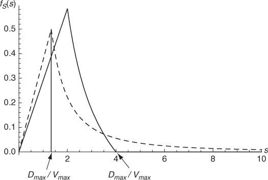
A final, fundamental observation made by Yoon et al. (2003) is that the pdf f_S(s) of the random variable S_i becomes heavy tailed when v_min → 0. The shape of f_S(s) is shown in Figure 5.8: the function increases linearly up to s = D_max/v_max; then, it starts decreasing till it reaches 0 when s = D_max/v_min. However, if v_min = 0 the right hand part of function f_S(s) never reaches 0, and the distribution is heavy tailed. In this case, E[S_i] becomes infinite, and v_RWP → 0. Thus, if v_min is set to 0, the stationary regime of a RWP mobile network actually coincides with a static network (v_RWP = 0), and is reached only after infinite time. It is clear then that setting v_min = 0, which is the default setting in popular wireless networks, might severely impact simulation accuracy and representativeness.

Figure 5.8 Shape of the pdf f_S(s) of random variable S_i for different speed values: v_max = 10 m/s, v_min = 5 m/s (solid curve), and v_max = 15 m/s, v_min = 0 m/s (dashed curve).

The intuitive explanation of the above result is the following: if v_min = 0, for a fixed arbitrarily small ϵ > 0, and the probability that a node chooses a speed in the range [0, ϵ]—near zero velocity—is a constant, then, by the law of large numbers, with infinite trials (trips) a near-zero velocity will eventually be chosen by every node in the network. When a near-zero velocity is chosen, the time needed to reach the destination, independently of its distance, approaches infinity. Thus, eventually each node in the network will get stuck in a trip with near-zero velocity, and the network will become virtually static.

5.4 Variants of the RWP Model

Several variants of the RWP model have been proposed in the literature, which we describe briefly in this section.

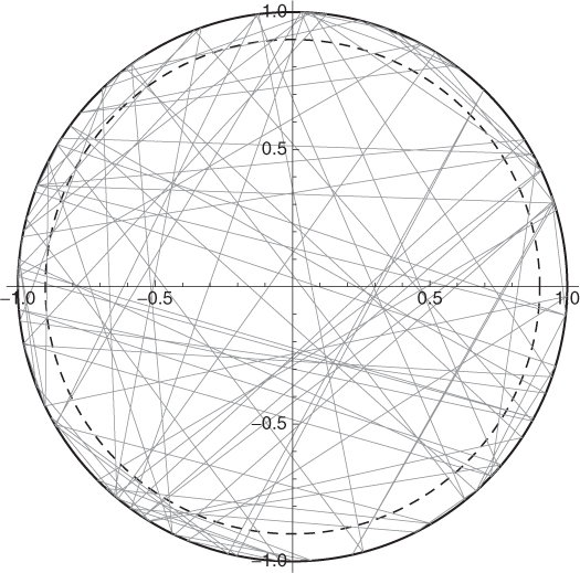
A variant of the RWP model, which is indeed a generalization, has been proposed by Bettstetter et al. (2003), where pause times are selected at each waypoint according to some probability distribution f_T(t) with bounded support. Several other variants of the basic model have been proposed by Hyytia et al. (2006). In particular, these authors assume that nodes move in a unit disk, and consider a variant of the RWP model in which the position of waypoints is chosen according to an arbitrary, rotationally symmetric distribution with support in the unit disk. An interesting sub-case of this variant is when waypoints are chosen uniformly at random on the border of the disk, which is named the RWPB (where B stands for border) in Hyytia et al. (2006). In other words, waypoints are chosen uniformly at random among the set of points at distance 1 from the center of the disk. These authors show that the stationary node spatial distribution in the RWPB model is relatively more concentrated on the border of the disk. This can be seen from Figure 5.9: the density of lines is relatively higher on the border (external annulus) than in the center of the square.

Figure 5.9 A hundred steps of RWPB mobility: the density of gray lines, representing trajectories, is relatively higher on the border (external annulus) than in the center of the disk.

References

Bettstetter C and Krause O 2001 On border effects in modeling and simulation of wireless ad hoc networks. Proceedings of the IEEE International Conference on Mobile and Wireless Communication Networks (MWCN), pp. 20–27.

Bettstetter C, Resta G and Santi P 2003 The node distribution of the random waypoint mobility model for wireless ad hoc networks. IEEE Transactions on Mobile Computing 2, 257–269.

Blough D, Resta G and Santi P 2002 A statistical analysis of the long-run node spatial distribution in mobile ad hoc networks. Proceedings of the ACM Workshop on Modeling, Analysis and Simulation of Wireless and Mobile Systems (MSWiM), pp. 30–37.

Hyytia E, Lassila P and Virtamo J 2006 Spatial node distribution of the random waypoint mobility model with applications. IEEE Transactions on Mobile Computing 5, 680–694.

Johnson D and Maltz D 1996 Dynamic source routing in ad hoc wireless networks. Mobile Computing, pp. 153–181. Kluwer Academic, Dordrecht.

Ns2Team 2011 http://www.isi.edu/nsnam/ns/.

Santaló LA 2002 Integral Geometry and Geometric Probability. Cambridge University Press, Cambridge.

Team G 2011a http://pcl.cs.ucla.edu/projects/glomosim/.

Team G 2011b http://www.ece.gatech.edu/research/labs/MANIACS/GTNetS/.

Yoon J, Liu M and Noble B 2003 Random waypoint considered harmful. Proceedings of IEEE Infocom, pp. 1312–1321.