Chapter 7

Random Trip Models

In this chapter, we will present and analyze the properties of a class of mobility models introduced in Le Boudec and Vojnovic (2006) called random trip models. This class of mobility models is very general, and includes most of the mobility models described in the previous chapters such as random walks and random waypoint, as well as many mobility models which will be described in forthcoming chapters. The importance of the class of random trip models lies in the fact that, if a mobility model is proved to belong to this class, fundamental model properties such as the existence and characterization of a stationary regime can be established based on the framework developed for the general class of random trip mobility models.

In what follows, we will first formally define the class of random trip mobility models, and present theoretical results derived by Le Boudec and Vojnovic (2006) concerning the existence and characterization of the stationary regime for a random trip mobility model. We will then conclude the chapter with specific instances of mobility models belonging to this general class.

7.1 The Class of Random Trip Models

Informally, a random trip is a model of random, independent node movements. Note that the requirement of independent movements implies that group mobility models do not belong to the class of random trip models. Formally speaking, the random trip model is defined by the notions of domain, phase, path, and trip, and by the definition of a default initialization rule:

1. Domain: the domain is a subset of , for some integer d ≥ 1, and represents the mobility region.

2. Phase: a phase is one of the possible states of the mobile node. Formally, represents the set of all possible phases in the model, where each element of can be thought of as an integer describing one of the (countably many) possible states of a mobile node. For instance, a phase in a random trip model might indicate whether the mobile node is currently moving or pausing at a certain location.

3. Path: a path represents a possible trajectory of a mobile node in , where is the set of all possible paths in . For instance, set might be the set of all line segments with both endpoints in , where is an arbitrary convex set. Formally, a path is a continuous mapping with a continuous derivative except possibly at a finite number of points. For any , P(0) is the starting point (origin) of the path, P(1) is the ending point (destination) of the path, and P(u), with u ∈ (0, 1), represents the position of a node in when a fraction u of its trajectory along path P is traversed.

4. Trip: a trip is defined by specifying a phase , a path , and a duration S_n, drawn according to some trip selection rule, specific to the model. For instance, in case only two phases (pause and move) are possible, the trip selection rule might dictate that a pause phase is always followed by a move phase, and that a move phase is always followed by a pause phase. Trip selection is performed at time instants T₀ ≤ 0 < T₁ < T₂ < …, where the are called transition instants. Given the phase I_n, the path P_n, and the duration S_n selected for the nth trip starting at time T_n, the next transition instant is T_n+1 = T_n + S_n. The position of a mobile node at time t, with T_n ≤ t ≤ T_n+1, is a continuous random variable taking values in , defined as

Note that the trip selection rule must always satisfy the property that P_n+1(0) = P_n(1), that is, the origin of the next path is the destination of the previous path. This is to avoid a mobile node being allowed to disappear from a point in and reappear soon after at another, possibly far-away, point in . For a similar reason, the duration S_n of a trip is constrained to take strictly positive values, that is, .

5. Default initialization rule: at time t = 0, representing the time at which observation of the mobile node starts, a phase, path, and remaining time till the next transition are drawn according to some initialization rule. The default initialization rule dictates that T₀ = 0 (i.e., the first transition instant occurs at time 0), and selects a phase, path, and trip duration according to the trip selection rule.

In order for a mobility model to belong to the class of random trip models, the following conditions on phase, path, and trip duration must be fulfilled. Note that a formal definition of these conditions is sometimes involved, requiring an understanding of non-trivial mathematical concepts. In what follows we have tried to simplify notation and presentation as much as possible, while only minimally sacrificing mathematical rigor. For a more rigorous definition of the conditions stated below, the reader is referred to Le Boudec and Vojnovic (2006).

7.1.1 Conditions on Phase and Path

The following conditions on phase and path must be satisfied:

1. Markov property: let Y = (Y_n), where Y_n = (I_n, P_n), be the stochastic process defined by observing the evolution of phase and path with time. Process Y must be a time-continuous, space-continuous Markov chain on . In particular, this means that process Y enjoys the Markov property (also called memory-less property): the state of the process at any time t > T_n depends only on the state of the process at the last transition instant T_n, and not on the state of the process at previous transition instants T₀, …, T_n−1.

2. Harris recurrent: the Markov chain Y must be Harris recurrent. The notion of Harris recurrence can be used to extend the notion of recurrence to Markov chains with continuous space state. When applied to the Markov chain Y = (I_n, P_n) at hand, conditions for Harris recurrence can be stated as follows. Let be the state space of Y. The Markov chain is Harris recurrent if there exist sets A, B ∈ Ω, a probability measure φ with support in B, and a number ϵ > 0 such that:

(a)

where .

(b)

where .

(c) If y ∈ A and C ⊂ B, then

Positive Harris recurrence implies that the measure π⁰ on Ω is such that , hence, it can be normalized to a probability measure, which represents the stationary probability distribution of the mobility model on the state space.

7.1.2 Conditions on Trip Duration

Random variables S_n describing trip duration must satisfy the following properties:

1. Independence of trip duration distribution: the distribution of trip duration S_n depends only on the current phase I_n and path P_n, and not on the history of past states (I₁, P₁), …, (I_n−1, P_n−1) and past durations S₁, …, S_n−1. Formally,

for any , and y ∈ Ω.

2. Positive trip duration: each trip takes a strictly positive time. Formally,

for any n ≥ 1 and y ∈ Ω.

3. A technical condition: in order to state the convergence in distribution to a time-stationary distribution for sample paths initialized at t = 0 according to the default initialization rule (recall Section 7.1, bullet point 5), it is required that the Markov renewal process defined by (Y_n, S_n), with n = 1, 2, …, is non-arithmetic. Since this condition is quite technical, we refer the reader to Le Boudec and Vojnovic (2006) for the formal definition. Informally, this condition is verified in case the distribution of random variable S_n has a density conditioned on a state set Y⁰ ⊂ Ω of strictly positive measure π⁰.

7.2 Stationarity of Random Trip Models

As mentioned at the beginning of this chapter, the importance of the class of random trip models lies in the fact that a formal characterization of necessary and sufficient conditions for the existence of a stationary regime has been derived for mobility models belonging to this class, as well as a characterization of the stationary state distribution in case a stationary regime exists. These results are summarized in the following theorem, derived by Le Boudec and Vojnovic (2006).

In what follows, the state of the mobile node at time t is described by the Markov process

where Y is the Markov chain describing the phase and path at time t, S(t) is the duration of the trip which is being undertaken at time t, and U(t) ∈ [0, 1] is the fraction of elapsed time on the current trip at time t.

Theorem 7.1 For a random trip model:

1. There exists a time-stationary distribution π for Φ if and only if the expected trip duration E(S₀) is finite. Whenever π exists, it is unique and defined as

for any . In the above formula, T₁ represents the first transition time after t = 0.

2. If E(S₀) is finite, then starting from the stationary distribution π⁰ of Markov chain Y for almost any trip at time 0, the process Φ(t) converges in distribution to π, as .

3. If E(S₀) is infinite, then

for any y ∈ Ω, and any set such that

Informally speaking, the theorem states that there exists a stationary regime for a random trip model if and only if the expected duration of a trip is finite, and characterizes the stationary distribution (conditions 1 and 2); if the expected trip duration is not finite (condition 3), then the Markov process is null-recurrent, that is, the mean number of transitions between successive visits to a regeneration set is infinite, and there exists no stationary regime.

7.3 Examples of Random Trip Models

In this section, we present examples of mobility models belonging to the class of random trip models. We start with an informal proof of the fact that the random waypoint mobility model is a random trip model (for the formal proof, see Le Boudec and Vojnovic (2006)). We then describe a few other mobility models which are shown in Le Boudec and Vojnovic (2006) to belong to the class of random trip models.

7.3.1 Random Waypoint Model

Let us consider the classical random waypoint mobility model on a convex region (say, on the unit disk). In order to prove that the model is a random trip model, we first have to define the domain, path, trip duration, and default initialization rule, and then prove the relative properties—recall Section 7.1.

1. Domain: the domain of mobility is the unit disk .

2. Phase: there are two possible phases, named I₁ = {pause} and I₂ = {move}.

3. Path: set is the set of all possible line segments with endpoints . Formally, a path is defined as , where P(u) = x₁(1 − u) + x₂u, where are the starting and ending points of the path, respectively. Special cases are those paths P_p for which x₁ = x₂, corresponding to pauses at a specific location. Denoting by the set of pause paths as defined above, we have that the support of random variable P_n is in if I_n = {pause}, while the support is if I_n = {move}.

4. Trip selection rule: the trip selection rule dictates that phases alternate between pause and move states. Formally, if I_n = {pause}, then I_n+1 = {move} and I_n+2 = {pause}. Trip duration S_n is drawn as follows. If I_n = {pause}, then S_n is chosen according to the pause time distribution F_pause(s). For instance, F_pause is the Dirac delta function centered at a certain pause time s_p > 0 in the standard random waypoint model. If I_n = {move}, the trip selection rule dictates that a point x_n+1 is chosen uniformly at random in , and that the selected path is the line segment connecting points x_n and x_n+1. To determine trip duration S_n, a speed V_n for the nth trip is chosen according to a distribution F_speed(v), for example, uniformly at random in an interval [v_min, v_max]. Trip duration S_n is then defined as:

where dist() denotes Euclidean distance.

5. Default initialization rule: the default initialization rule dictates that a mobile node starts in pause time, at a location x₀ chosen uniformly at random in .

We now verify that conditions on phase, path, and trip duration are fulfilled.

1. Markov property: the stochastic process defined by Y_n = (I_n, P_n) is clearly a Markov chain: the next phase I_n+1 depends only on the previous phase I_n, and the distribution according to which path P_n is drawn depends only on I_n.

2. Harris recurrence: to prove Harris recurrence of Markov chain Y_n, it is sufficient to take set as the recurrent set, to choose φ = Unif⊗Unif (product measure) as the probability measure on A, and to set ϵ to an arbitrary positive value—see Le Boudec and Vojnovic (2006) for a formal proof.

3. Positive Harris recurrence: to prove positive Harris recurrence, it is sufficient to observe that the recurrent set A is visited at each transition.

4. Independence of trip duration distribution: the distribution of trip duration depends only on the current phase I_n, so the property is satisfied.

5. Positive trip duration: if in pause phase, trip duration is set to s_p > 0; otherwise, it is a positive quantity determined by the ratio of two strictly positive numbers. In both cases, trip duration is strictly positive.

6. Technical condition: the technical condition is also satisfied, since random variable S_n has a density.

Since the expected duration of a trip in the random waypoint model is clearly finite, we have that, according to Theorem 7.1, the random waypoint model has a uniquely defined stationary regime. Note that the stationary regime as defined within the context of random trip models includes both the stationary node spatial distribution (given by random variable X(t) defined as in Section 7.1) and the node speed. Thus, the framework of random trip models can be seen as a more formal way of characterizing the node spatial distribution and average nodal speed of the random waypoint model which were described in Chapter 5.

7.3.2 RWP Variants

Several variants of the random waypoint mobility model have been proved in Le Boudec and Vojnovic (2006) to belong to the class of random trip models:

• The Swiss flag mobility model: in this mobility model, the domain is a non-convex set corresponding to the interior of a Swiss cross—see Figure 7.1. The set of phases is the same as in the original random waypoint model. The set of paths when in move phase is the set of shortest paths between any two points , where the path is entirely inside —see Figure 7.1. The set of pause paths is defined as in the original random waypoint model. The trip selection rule chooses a new endpoint uniformly in , and the next path is the shortest path from the current to the next endpoint. In case there are several such paths, one of them is selected uniformly at random. The rules for trip duration selection are the same as in the original random waypoint model.
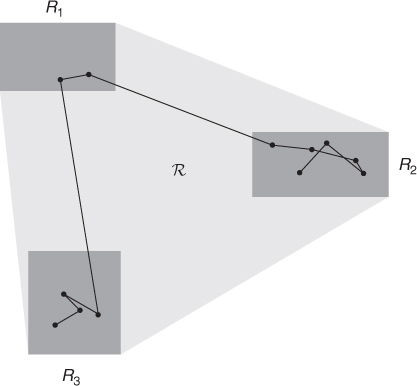
• The restricted random waypoint model: the model was originally introduced in Blazevic et al. (2004), but it is defined in a more general way in Le Boudec and Vojnovic (2006). In this model, the domain is the convex closure of a set of convex sub-domains R₁, …, R_k—see Figure 7.2. Trip endpoints are chosen in the sub-domains R_i according to the following rule. Suppose the node starts from a point x₀ ∈ R_i. The number r of trip endpoints to be chosen in R_i is selected according to a probability distribution F_i(), specific to the sub-domain. For the next r trips, endpoints are chosen uniformly at random in R_i. After the rth trip, a new sub-domain R_j, with j possibly equal to i, is chosen according to a probability distribution F_{domain, i}(). The destination for the (r + 1)th trip is chosen uniformly at random in R_j, and the path from the last destination in sub-domain R_i to the first destination in R_j is a line segment. The rules for trip duration selection are the same as in the original random waypoint model.
• The random waypoint on sphere: this is a version of the random waypoint model in which the domain is the surface of the unit sphere in . The path between two endpoints x₁, x₂ (chosen uniformly at random on the surface of the sphere) is the shortest of the arcs on the circle of unit radius passing through x₁, x₂. If the two arcs have the same length, one of them is chosen uniformly at random. Rules for trip duration selection are as in the original random waypoint model.

Figure 7.1 The Swiss flag mobility model. Depending on the position of endpoints, a path can be composed of either one or two linear segments.

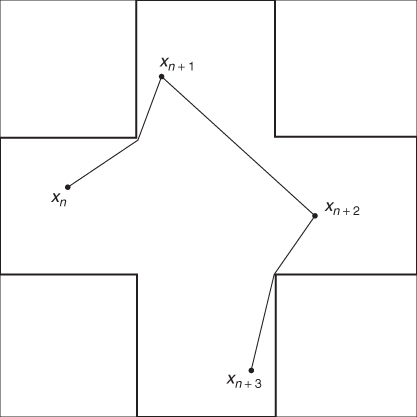
Figure 7.2 The restricted waypoint mobility model with three mobility sub-domains.

7.3.3 Other Random Trip Mobility Models

These are as follows:

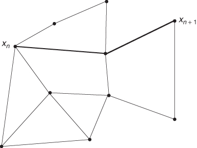
• Space graph model: in this model, originally introduced in Jardosh et al. (2003), there exists a set from which waypoints are chosen, corresponding to the set of possible destinations on a map. The mobility domain corresponds to the union of R₁ with the edges of the planar graph connecting the points in R₁—see Figure 7.3. The rules for trip selection are similar to that of the restricted waypoint mobility model with a single mobility sub-domain. This model is very similar to the vehicular mobility model introduced in Tian et al. (2002).
• Random walk on torus: this is the classical time- and space-continuous random walk model on a bounded domain (say, a rectangle), where a wrap-around border rule is used. The trip selection rule dictates that a speed vector V_n and a trip duration S_n are chosen independently, according to some time-invariant probability distributions.

Figure 7.3 The space graph mobility model: waypoints are nodes in a spatial graph; trajectories correspond to shortest paths in the spatial graph.

References

Blazevic L, Le Boudec JY and Giordano S 2004 A location-based routing method for mobile ad hoc networks. IEEE Transactions on Mobile Computing 3, 97–110.

Jardosh A, Belding-Royer E, Almeroth J and Suri S 2003 Towards realistic mobility models for mobile ad hoc networking. Proceedings of the ACM International Conference on Mobile Computing and Networking (MOBICOM), pp. 217–229.

Le Boudec JY and Vojnovic M 2006 The random trip model: Stability, stationary regime, and perfect simulation. IEEE/ACM Transactions on Networking 14, 1153–1166.

Tian J, Hahner J, Becker C, Stepanov I and Rothermel K 2002 Graph-based mobility model for mobile ad hoc network simulation. Proceedings of the ACM/IEEE Annual Simulation Symposium, pp. 337–344.