Chapter 10

WLAN Mobility Models

Mobility models for WLAN environments can be broadly classified into two categories. The first category comprises models whose goal is to closely resemble user/AP registration patterns observed in WLAN traces. Models in this category, such as those presented in Jain et al. (2005), Lee and Hou (2006), Lelescu et al. (2006), Chinchilla et al. (2004), and Tuduce and Gross (2005), can be used, for instance, to predict the next user AP association given the current association. Physical user mobility in these models is then not explicitly modeled, although it can be deduced from a user's AP association pattern. The second category of models is instead aimed at modeling user physical mobility. In this case, the history of a user's AP associations is used to generate a realistic trace of the user's physical mobility in the environment. By aggregating traces of several users, a statistical model of user physical mobility in the WLAN environment can be derived and used to faithfully reproduce the physical movement of users. Examples of models in this category are given in Hsu et al. (2004) and Kim et al. (2006).

In this chapter, we will present two representative mobility models for each of these two categories of WLAN models. More specifically, we will present:

Before proceeding further, a comment is in order about the motivating reasons for designing WLAN mobility models. In contrast to other application scenarios, a relatively large number of real-world WLAN traces nowadays are publicly available and can be used to test the performance of WLAN algorithms/protocols. Despite this, synthetic models able to generate realistic WLAN traces are very useful, since they allow changes in parameters and network configuration (e.g., growing the number of users beyond the maximum number registered in a WLAN trace, or increasing the number of APs in the network), which are only partially possible if an existing real-world trace is used instead.

10.1 The LH Mobility Model

The LH model was introduced by Lee and Hou (2006) to faithfully reproduce WLAN traces. Different from other existing models, the LH model attempts to predict not only the most probable AP association given the current user association, but also the time at which the transition will take place. Bringing the temporal dimension into the model was a major advance with respect to the state of the art.

As in other approaches, the LH model uses Markov chains to model transitions between the APs in the network. However, the model introduces a temporal dimension in the Markov chain by including a parameter that models the time at which transitions between APs take place.

More formally, given a network composed of m APs, which we assume to be numbered from 1 to m, the behavior of a user in the network is modeled by the following semi-Markov model:

where X_n ∈ {1, …, m}∪{0} is the nth user association, called state in the following, and T_n is a continuous random variable taking values in [0, + ∞) representing the time at which the transition between state X_n−1 and state X_n takes place (T₀ = 0). Note that the set of possible states is augmented with state 0, modeling a user who is currently disconnected from the WLAN (recall the discussion in Section 9.2).

The model described is a semi-Markov chain, since the distribution of random variable T_n is not exponential; instead, Lee and Hou (2006) make no specific assumption about the distribution of T_n, which is empirically derived from the analysis of an existing WLAN trace. Their choice of not assuming an exponential distribution for variable T_n is motivated by the observation, first made by Balazinska and Castro (2003) and reported in the previous chapter (see Figure 9.2), that the session duration distribution is a power law. Lee and Hou, however, make the assumption that the semi-Markov process is time homogeneous: that is, the distribution of random variable T_n does not change during the period in which the mobility model is built.

In order to fully characterize the previously defined semi-Markov chain, the following transition probabilities need to be evaluated:

where P(X_n+1 = j, T_n+1 − T_n ≤ t|X_n = i) is the probability of making a transition to state j within time t starting from state i, p_ij = lim_t→∞Q_ij = P(X_n+1 = j|X_n = i) is the state transition probability between states i and j (independent of transition time), and H_ij(t) = P(T_n+1 − T_n ≤ t|X_n+1 = j, X_n = i) is the sojourn time in state i when the next state is j.

Note that the semi-Markov chain model allows great flexibility in modeling sojourn time at APs, since different sojourn time distributions can be used depending on the specific transition the user will perform. In other words, the sojourn time distribution when the user is associated with AP i and the next state is known to be AP j is in general different from that when the user is known to make a transition to another AP z ≠ j starting from i.

Let D_i(t) denote the probability distribution of the sojourn time in state i, independently of the next state. It can be seen that

Given D_i(t), the homogeneous semi-Markov chain modeling WLAN user behavior can be formally defined as , with transition distributions defined as

In this formula, ϕ_ij(t) must be interpreted as the probability of finding a user in state j after time t, starting from state i, and δ_ij is the Kronecker delta function defined as

10.1.1 Estimating the Transition and Steady-State Probabilities

In order to define the semi-Markov chain modeling user behavior, the following quantities need to be derived:

The above values have been estimated in Lee and Hou (2006) by analyzing wireless network traces collected at Dartmouth College between November 1, 2003, and June 30, 2004, and available through the CRAWDAD website (Team 2011). The traces comprise data collected from 586 APs all over the 161 buildings of the Dartmouth College campus, and refer to 6202 tracked users in total.

Based on the estimated transition probabilities and sojourn time distributions, it is possible to estimate the steady-state user distribution, that is, the probability π_i of finding a user in state i at a random (and very large) instant of time t, as follows:

where is the average sojourn time in state x, and is the steady-state probability of making a transition to state x, which can be found by solving the following set of equations:

where is the vector of steady-state transition probabilities, and P = [p_ij] is the matrix of transition probabilities p_ij.

As we will see next, characterization of the steady-state distribution of users across APs allows evaluation of the temporal correlation between user and AP association patterns.

10.1.2 Finding Temporal Correlation in User/AP Association Patterns

The steady-state user distribution across APs can be used to investigate whether, and to what extent, mobility patterns are correlated in time. The basic idea is to compute the steady-state distribution at different time intervals (e.g., a day, a week, or a month), and to use a similarity metric to estimate the degree of similarity between the distributions computed at the different time intervals. Since the steady-state distribution of users across APs is represented by an (m + 1)-dimensional vector , Lee and Hou (2006) suggest using a vector similarity metric, the cosine distance, to express the similarity between distributions.

The cosine distance metric is defined as follows. Let A and B be two n-dimensional vectors. The cosine distance between A and B, denoted sim(A, B), is computed as

If both A and B lie in the first quadrant of Euclidean space (as is the case with probability distributions, which can take only positive values), the cosine similarity metric takes values in [0, 1], with sim(A, B) = 0 expressing minimal similarity between the vectors (orthogonal vectors), and sim(A, B) = 1 corresponding to maximal possible similarity (identical vectors).

Before proceeding to estimate temporal correlations, Lee and Hou (2006) observed that, in order to obtain estimates of sojourn time distribution that accurately reflect user mobility behavior, a certain number of AP transitions not related to mobility must be removed from the traces. These transitions, called ping-pong transitions, might occur if a user is located in a position covered by multiple APs. In this situation, due to phenomena such as changes in network traffic load, changes in the radio environment, etc., a user's association can change even if the user is not physically moving. However, identifying ping-pong transitions in the trace is relatively easy, since they generate repetitive association patterns.

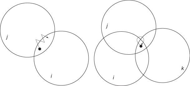
Lee and Hou (2006) classify ping-pong transitions as either i → j → i → j or i → j → k → i form (corresponding to a user lying within the coverage areas of two or three different APs, respectively—see Figure 10.1). The ping-pong transitions are then removed from the traces by associating a user with the prevalent AP for the entire duration of the ping-pong transition, where the prevalent AP is defined as the AP with which the user spends most of the time during the ping-pong phase.

Figure 10.1 Examples of ping-pong transitions when the user is in the coverage area of two (left) or three (right) APs.

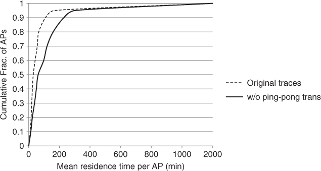
An important observation made by Lee and Hou (2006) is that ping-pong transitions do occur frequently in WLAN traces (at least the ones analyzed by the authors): on average, about one-third of a user's transitions are indeed ping-pong transitions, and should be removed from the trace. If ping-pong transitions are not removed, the sojourn time distribution at APs can be erroneously underestimated. The effect of ping-pong transitions on sojourn time distribution is evident in Figure 10.2, showing the distribution of the mean residence time at APs derived from the original traces, and after removal of ping-pong transitions. The mean and median AP residence times are 51 minutes and 33 minutes, respectively, in the original data; after removal of ping-pong transitions, these times increase to 108 minutes and 73 minutes, respectively.

Figure 10.2 The distribution of mean residence time at APs before and after removal of ping-pong transitions.

Let us now evaluate the similarity in user mobility at different time scales. In particular, Lee and Hou (2006) considered three time intervals: day, week, and month. For each time interval, these authors divided the original trace into a number of sub-traces of the corresponding interval. For instance, when considering monthly correlation in user mobility, the authors divided the trace into eight sub-traces, each corresponding to a different month. The steady-state distribution of users across APs is then computed for each sub-trace, giving a number k of different steady-state distributions , respectively. For each pair , the cosine distance between and is then computed. Intuitively, if the cosine distance turns out to be relatively close to 1, this implies that user mobility (more specifically, the distribution of users across APs) in time interval i is very similar to user mobility in time interval j, that is, user mobility patterns tend to repeat themselves in the time scale of interest (day, week, or month).

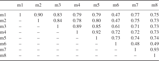
The cosine distance values for all possible pairs of monthly sub-traces derived from the eight month-long original data traces are given in Table 10.1. It is interesting to observe that the degree of similarity between monthly sub-traces is in general very high, especially for consecutive months. A relatively lower correlation value is displayed between sub-trace m6 and the other traces, which can be explained by the fact that this sub-trace contains the week corresponding to the spring break. Based on the results in Table 10.1, Lee and Hou (2006) conclude that user mobility displays a high degree of monthly correlation. Similar conclusions are drawn for daily and weekly correlation in user mobility patterns—see Lee and Hou (2006) for details.

Table 10.1 Monthly correlation in WLAN user mobility reporting, for each pair of monthly sub-traces, the cosine distance of the corresponding steady-state user/AP distribution

10.1.3 Timed Location Prediction with the LH Model

While the characterization of the steady-state distribution of users across APs can be used to reveal interesting time correlation properties of user mobility patterns, it cannot be directly used to predict the most likely next association (also called location) of a user, given her/his current association. Location prediction is an important feature of a WLAN mobility model that can be used, for example, for network resource provisioning, network traffic load balancing, etc.

Lee and Hou (2006) present a methodology for location prediction based on the derived semi-Markov chain model. Indeed, the methodology allows estimation of not only the most probable next location given the current AP association, but also the most likely session duration at the current AP. The methodology used to derive location and session duration predictions is quite involved, so in the following we only summarize the intuition behind it. The interested reader can find details in Lee and Hou (2006).

In order to predict the next location and session duration, the transition probabilities ϕ_ij(t) of the semi-Markov chain must be estimated. We recall that ϕ_ij(t) represents the probability of finding the user in state j at time t, given that the user was in state i at time 0.

Estimating probabilities ϕ_ij(t) is a quite difficult task, which Lee and Hou (2006) tackle by considering a time-discrete approximation of the original transition probabilities. More specifically, these authors assume that time is discretized into relatively small time intervals of size h, and estimate transition probabilities ϕ_ij(k), corresponding to the probability of finding a user in state j at time t = k · h, given that the user was in state i at time 0. Time discretization is used also to estimate the distributions required to compute ϕ_ij(k), namely, Q_ij(kh) (transition probability between states i and j, independently of transition time) and D_i(kh) (distribution of residence time in state i, independently of next location). Also, the distribution H_ij(kh) (distribution of residence time in state i, given that next state is j), which is needed to estimate sojourn time at the current AP, is estimated through time discretization.

In order to estimate the transition probabilities, the following procedure is performed whenever a transition between state i and j occurs:

Here K is the number of bins used to approximate the probability distributions.

The accuracy of the timed location prediction methodology has been evaluated in Lee and Hou (2006) using the Dartmouth WLAN trace. Every T_p seconds, where T_p is a tunable parameter, the semi-Markov mobility model is used to make predictions about the next possible state. When performing predictions, those made in the OFF state are not considered when collecting accuracy statistics. In fact, users tend to remain in the OFF state for a relatively long period of time, and estimating the next most likely state when a user is in the OFF state is a trivial task that succeeds most of the time, thus leading to an overestimate of the actual prediction accuracy.

Two methods are suggested to evaluate prediction accuracy: the 1-location estimator, according to which the next AP corresponds to the AP with the highest transition probability; and the 2-locations estimator, which considers also the AP corresponding to the next highest transition probability as a second possible next state. Note that also the current AP can be included in the outcome of the location estimators, corresponding to the situation in which no transition actually takes place.

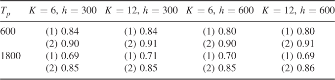
The accuracy of the two location estimators described above for different values of the time discretization parameters h, K and estimation period T_p are given in Table 10.2. As can be seen from the table, the accuracy is quite high, especially for the 2-locations estimator.

Table 10.2 Prediction accuracy of the 1-location (1) and 2-locations (2) estimators for different values of the time parameters. Values of T_p, h, and K are expressed in seconds

10.2 The KKK Mobility Model

In contrast to the LH model described in the previous section, the mobility model introduced in Kim et al. (2006) has the goal of modeling the physical movement of users within the environment. More specifically, the KKK model is designed to generate synthetic trajectories in a physical space resembling those observed in a large WLAN covering a university campus. Since the physical movement of users is not directly traced in collected WLAN data, but only the history of their AP associations, a first difficulty faced by these authors was extracting a reasonably accurate trajectory of a user's movement starting from the AP associations trace. The analysis of the salient features of these user trajectories allowed Kim et al. (2006) to derive a relatively simple synthetic model generating trajectories with similar features.

10.2.1 Extracting Physical Movement Trajectories from WLAN Traces

Extracting a physical movement trajectory from an AP association trace is a very challenging task. First of all, as we commented in Chapter 9, most WLAN users are indeed nomadic, rather than mobile: different from a mobile user, a nomadic user uses the WLAN device while residing in a certain place for a relatively long time; this user can then move to a different location (where she/he will also likely spend a relatively long time), but typically the WLAN device is turned off during the traveling phase. Thus, extracting accurate physical movement trajectories from traces of nomadic users is very difficult, essentially due to lack of data.

To get around this difficulty, Kim et al. (2006) decided to base their model only on the observation of a specific class of users, namely, VoIP users: in fact, unlike other classes of WLAN users, VoIP users are likely to behave as mobile (i.e., having the VoIP device turned on also during the traveling phase), instead of nomadic, entities. More specifically, the Kim et al. (2006) considered a trace referring to 198 VoIP users collected at Dartmouth College in a 13-month period from the beginning of June 2003 to the end of June 2004.

Even if only mobile users are traced, extracting a physical movement trajectory from an AP association trace remains a difficult task. The most intuitive methodology for transforming AP traces into a physical movement trajectory would be to locate the user in the vicinity of the AP she/he is registered with. Unfortunately, directly applying this methodology would work poorly, since the AP a user is registered with is not necessarily the closest one to the user. In fact, APs might use different power levels to transmit; even if the same transmit power level were set in all APs, radio signal propagation in the environment would be highly heterogeneous, possibly leading a user to get better signal quality from a relatively far-away AP. Finally, different network interfaces might have different aggressiveness in changing associations from a relatively weak to a relatively strong AP: if the network card is not very aggressive, the current AP association can be retained for a relatively long time, even if an AP with much better signal quality is available.

Kim et al. (2006) suggest three methods for extracting a physical movement trajectory from an AP trace, all of which build upon the fact that the exact (x, y) coordinate of each AP on the Dartmouth College campus is known and reported in the traces:

Figure 10.3 Estimated user position using the triangle centroid (left) and time-based centroid (right) algorithms.

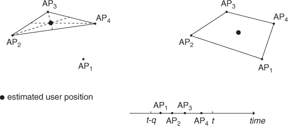
By comparing the physical trajectories derived from the above algorithms to a few GPS traces obtained from volunteers moving on the campus, Kim et al. (2006) conclude that the Kalman filter is the most accurate method, and it is then used to extract physical movement trajectories from the WLAN data traces.

Before extracting the physical trajectories, Kim et al. (2006) pre-processed the traces in order to distinguish between relatively mobile and relatively stationary sub-traces. First of all, for each user, only data collected within working hours (defined as the interval between 8 AM and 6 PM) is considered. Then, the authors classified each workday sub-trace as either mobile or stationary according to the following criterion: for each workday, the maximum Euclidean distance (diameter) between the locations of any two APs occurring in the sub-trace is computed. A workday sub-trace is then classified as stationary if its diameter is less than 100 m, otherwise it is classified as mobile. The analysis of the whole trace reveals that only 46% of the workday sub-traces are classified as mobile.

10.2.2 Extracting Pause Time

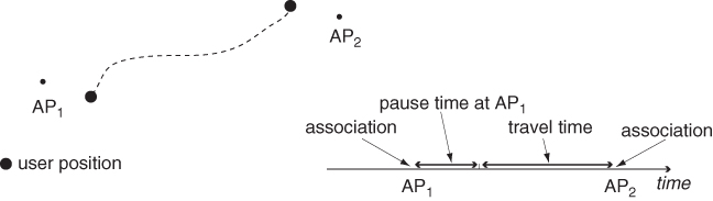
Another task to be accomplished in the process of extracting physical movement trajectories from WLAN traces is accurately estimating the pause time at the various locations. In other words, the time elapsing between a user's association with access point AP₁ and her/his next association with AP₂ must be broken down into a pause time at AP₁, followed by a travel time from AP₁ to AP₂ (see Figure 10.4).

Figure 10.4 Breakdown of a time interval into pause time at an AP and travel time between two consecutive APs.

The algorithm proposed in Kim et al. (2006) to estimate pause times is as follows. The “raw” user speed when moving from access point AP₁ to the next access point AP₂ is computed as

where |l₂ − l₁| is the Euclidean distance between AP₂ and AP₁, and t_i is the time of association with access point AP_i.

The raw user velocity is then compared to a “normal” speed range estimated from the assumption that the user is a pedestrian. More specifically, the normal speed range is defined as the interval [min, 10] m/s, where two possible values of min (0.1 and 0.5 m/s) are considered in Kim et al. (2006). If v_r is within normal range, then it is assumed that the user did not stop at AP₁, but was simply traveling between AP₁ and AP₂ during time interval t₂ − t₁ (i.e., pause time at AP₁ is assumed to be 0). If the raw speed v_r is above the normal speed, it is assumed that the change in AP association is not reflecting a real user movement, and that portion of the trace is discarded. Finally, if the raw speed is below the normal speed, a pause time at AP₁ is computed as follows:

where is the average speed of the user, which is computed as an exponentially weighted moving average; more specifically,

where is the user average speed as computed in the previous segment of the trajectory.

Kim et al. (2006) then proposed a heuristic to aggregate consecutive pause times in case the location of a user remains confined within a relatively small range (called clustering range)—see Kim et al. (2006) for details.

Similar to the physical trajectory extraction method, the pause time extraction algorithm is evaluated in Kim et al. (2006) by comparing the estimated pause times to ground truth data obtained from a few volunteers performing a pause time+travel trip within the Dartmouth campus. The comparison reveals the efficacy of the proposed algorithm extended with the clustering range heuristic in estimating pause times.

10.2.3 Dealing with Stationary Sub-Traces

The methods described to extract physical movement trajectories and pause times are relevant only for mobile sub-traces. For stationary sub-traces, the degree of user movement is so low (recall that a workday sub-trace is classified as stationary if its diameter is less than 100 m) that the user recorded in the trace is assumed to be stationary for the entire duration of the trace. Thus, determining user location and pause time is a relatively easy task in this case: the user location is determined according to the triangle centroid method and remains fixed for the entire duration of the sub-trace; accordingly, the pause time at the estimated location is assumed to be equal to the duration of the sub-trace.

10.2.4 Finding Hotspot Locations

A final ingredient of the KKK mobility model is the definition and positioning of hotspot locations, namely, popular locations. For mobile sub-traces, the authors identify hotspot locations within the Dartmouth College campus using a simple technique that builds upon the definition of pause time: whenever a user pauses at an AP, a 2-D Gaussian distribution of “popularity weight” is applied at the current user location, thus creating a small “popularity mountain” centered at the user's location. The “height” of the mountain (peak of the Gaussian distribution) is directly proportional to the pause time duration. Popularity mountains for each visit are then added up across all users, and hotspot regions are identified as those region of the space where the popularity weight is consistently higher than a certain threshold (see Kim et al. (2006) for details). In the case of stationary sub-traces, the 2-D Gaussian distribution is not weighted with the duration of the stay at the current (fixed) location.

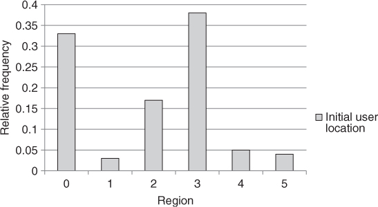
Based on the analysis of data reported in both mobile and stationary sub-traces, Kim et al. (2006) identify five hotspot regions on the Dartmouth College campus, corresponding to the School of Engineering, the main Dartmouth Library, the Computer Science Department, the office building of campus network administrators, and a hotel containing a restaurant (see Figure 10.5). The distribution of the initial user location across the five hotspots is displayed in Figure 10.6, with region 0—called the cold region—modeling an initial location anywhere outside the five hotspot regions. As can be seen from the figure, approximately 67% of the users start their walk from a hotspot region.

Figure 10.5 Dartmouth College campus map with the locations of the five hotspot regions.

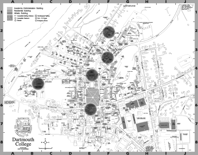
Figure 10.6 Distribution of initial user location across hotspots.

The definition of hotspot regions is also useful for characterizing movement between the hotspots. More specifically, based on WLAN data traces, an n × n transition matrix M can be computed, with element m_ij corresponding to the probability of moving to location j starting from location i. Note that the transition matrix includes not only the five hotspots and the cold region, but also a “virtual” location corresponding to the OFF state.

10.2.5 Mobility Modeling

Based on the above-described algorithms for physical movement trajectory extraction, pause time characterization, and hotspot localization, the following model for synthetically generating user trajectories is defined in Kim et al. (2006):

Figure 10.7 Generation of the mobility trace starting from an initial location i and the final location j.

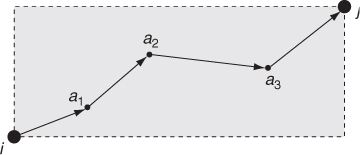
Table 10.3 Probability distributions used in the KKK mobility model. The pause time and speed distributions are derived using min = 0.1 m/s

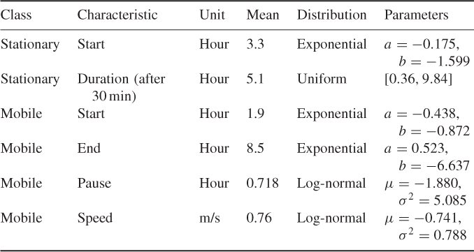
The distributions used to generate the start and end times of the trace, duration of the stay and pause time, and movement speed, are derived from an analysis of the WLAN data trace, and are summarized in Table 10.3.

We recall that the exponential distribution is defined by the following pdf:

and the log-normal distribution is defined by the following pdf:

Kim et al. (2006) validate the KKK model against the WLAN data trace. Clearly, to validate the model a mobility parameter different from those used to define the model itself should be used. The authors use the number of visitors within a certain region in each hour of the workday as a relevant parameter, and validate the KKK model by comparing visitor numbers as computed from a synthetic KKK trace to those derived from the WLAN data trace. They find that the KKK model generates reasonably accurate movement traces, with the median relative error in estimating visitor numbers around 17%.

10.3 Final Considerations and Further Reading

In this chapter, we have presented two relevant mobility models for WLAN environments. Besides acquainting the reader with two specific mobility models, the aim of this chapter was to give also an idea of the probabilistic/statistical tools and methodologies used to extract a mobility model from WLAN data traces.

As the reader might have noticed, extracting a mobility model from WLAN traces is not a trivial task, because it requires a significant amount of pre- and post-processing of the traces, as well as considerable modeling efforts. Yet, it is possible to define synthetic trace generators able to faithfully reproduce traces observed in a certain WLAN environment. On the downside, the models described in this chapter—as well as the other WLAN mobility models introduced in the literature—are representative only of the specific WLAN environment from which they are derived, namely, different traces collected on the Dartmouth College campus. If the goal of a network designer were to model mobility in a different WLAN environment—say, a different campus, or a corporate instead of university WLAN—a different tuning of the model parameters, if not a complete redefinition of the models, would be required.

As commented briefly at the beginning of this chapter, several other mobility models derived from WLAN trace analysis have been proposed in the literature. Among the most representative ones, we cite the Model T and Model T++ models introduced in Jain et al. (2005) and Lelescu et al. (2006), respectively, and the model introduced in Tuduce and Gross (2005). The reader interested in gaining a better understanding of WLAN mobility modeling can start from these models.

References

Balazinska M and Castro P 2003 Characterizing mobility and network usage in a corporate wireless local-area network. Proceedings of ACM MobiSys.

Chinchilla F, Lindsey M and Papadopouli M 2004 Analysis of wireless information locality and association patterns in a campus. Proceedings of IEEE Infocom.

Hsu WJ, Merchant K, Shu HW, Hsu CH and Helmy A 2004 Preference-based mobility model and the case for congestion relief in WLANs using ad hoc networks. Proceedings of the IEEE Vehicular Technology Conference (VTC), Fall.

Jain R, Lelescu D and Balakrishnan M 2005 Model T: An empirical model for user registration patterns in a campus wireless LAN. Proceedings of the ACM International Conference on Mobile Computing and Networking (MOBICOM), pp. 170–184.

Kim M, Kotz D and Kim S 2006 Extracting a mobility model from real user traces. Proceedings of IEEE Infocom.

Lee JK and Hou J 2006 Modeling steady-state and transient behaviors of user mobility: Formulation, analysis, and application. Proceedings of the ACM International Symposium on Mobile Ad Hoc Networking and Computing (MobiHoc), pp. 85–96.

Lelescu D, Kozat U, Jain R and Balakrishnan M 2006 Model T + + : An empirical joint space-time registration model. Proceedings of the ACM International Conference on Mobile Ad Hoc Networking and Computing (MobiHoc), pp. 61–72.

Team C 2011 http://crawdad.cs.dartmouth.edu/index.php.

Tuduce C and Gross T 2005 A mobility model based on WLAN traces and its validation. Proceedings of IEEE Infocom, pp. 664–674.