Chapter 13

Microscopic Vehicular Mobility Models

In the previous chapter we saw how the problem of modeling vehicular mobility can be addressed at different geographical scopes, namely, at a macroscopic and microscopic level. In this chapter, we will focus our attention on the class of microscopic mobility models, which are by far the most relevant in the simulation of vehicular network performance.

We start by presenting three simple microscopic models, which can be thought of as relatively simple extensions of the well-known random walk and random waypoint mobility models. More specifically, we will present the graph-based mobility model introduced in Tian et al. (2002), and the Freeway and Manhattan mobility models introduced in Bai et al. (2003). Then, we will describe in detail a more complete model, the SUMO model, developed and maintained by the Institute of Transportation Systems at the German Aerospace Center. Unlike the models mentioned earlier, SUMO comprises tools for the automatic acquisition of digital road maps from different sources, and very accurate traffic rule and driver behavior modeling. Finally, in the last part of the chapter we will discuss the challenges related to accurately simulating both vehicular mobility and wireless communication, and present a representative tool aimed at effectively integrating vehicular mobility and wireless communication simulation.

13.1 Simple Microscopic Mobility Models

13.1.1 The Graph-Based Mobility Model

The graph-based mobility model was introduced in Tian et al. (2002) to model the mobility of humans in a urban environment. Although the model was originally defined for pedestrian mobility, it can be extended to model vehicular mobility in a straightforward way.

The first step in the graph-based mobility model is the definition of a graph representing all possible paths in the simulated region. More specifically, the vertices of the graph represent locations that mobile nodes can visit—corresponding to points of interest in vehicular mobility modeling terminology—while the edges represent connections between these locations. Connections are defined in a quite abstract way in this model, and could be intended for instance to represent pathways between buildings on a campus in case pedestrian mobility is modeled, or roads if the goal is to model vehicular mobility.

Tian et al. (2002) assume that the path graph is given as input to the model, and that it is a connected graph. The path graph can be either randomly generated or extracted from a map of the region of interest. An example of a randomly generated path graph is shown in Figure 13.1.

Figure 13.1 Example of a randomly generated path graph modeling a city center, and of a trip between randomly chosen source and destination.

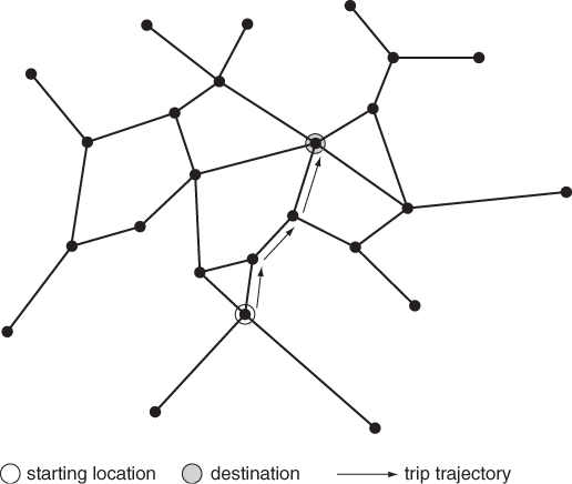
The second step in the mobility simulation process consists of generating the initial positions of mobile nodes, which are assumed to be located at a randomly chosen vertex in the path graph. Once initial positions are chosen, nodes start moving according to a random waypoint-like pattern—see Figure 13.1:

While the graph-based mobility model accounts for geographically constrained movements and, in this respect, can be considered an improvement over other synthetic mobility models such as random walk and random waypoint, the model does not account for the other two distinguishing features of vehicular mobility described at the beginning of Chapter 12, namely, traffic rules and driver behavior. The models presented next take a step forward in accurate vehicular mobility modeling, since they also include simple traffic rules in the model definition.

13.1.2 The Freeway Mobility Model

The freeway mobility model was introduced in Bai et al. (2003) to model the movement of vehicles along a freeway. Similar to the graph-based mobility model, the model takes as input a map of freeways in the region of interest. Multi-lane freeways are modeled using parallel edges, as shown in Figure 13.2. The freeway map can be either extracted from a real map, or randomly generated.

Figure 13.2 Example of freeway map and corresponding ingress/egress points in the freeway mobility model.

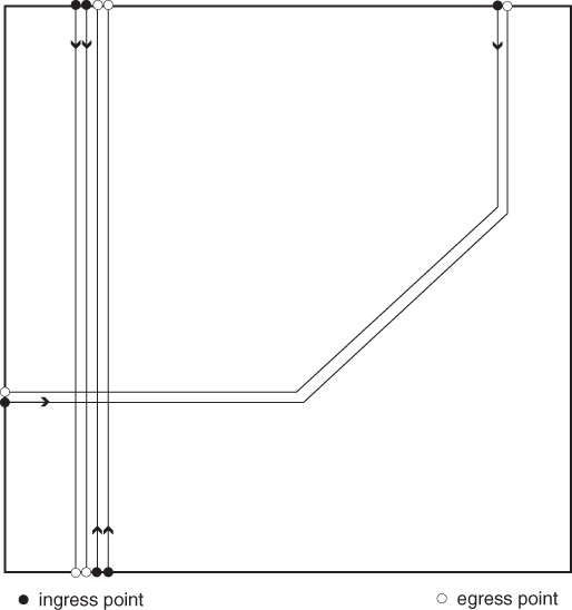
The freeway map input implicitly defines ingress and egress points, that is, points where vehicles enter and leave the simulated region, as in the figure. Vehicles enter the simulated region from a randomly chosen ingress point (corresponding to a freeway lane), then they move along the selected lane until they exit the simulated region from the corresponding egress point. It is important to observe that, while freeway lanes are allowed to cross each other in the map (see Figure 13.2), these crossings do not represent junctions that can be used to enter in a different lane.

Since no rules for lane changing are defined in the model, the velocity of a vehicle is strongly related to the velocity of the preceding vehicles in the same lane—that is, a car-following rule is defined. Furthermore, in order to improve the realism of the model, the current velocity of a vehicle is made dependent also on its velocity at the previous time step (note that the freeway mobility model is a discrete-time mobility model).

More formally, the rules used for determining a vehicle's velocity are as follows:

The car-following rule must be interpreted as imposing an upper bound on the velocity chosen using the first rule: if the chosen velocity of a vehicle according to this rule for the next time step is v_i and the vehicle is within the safety distance of a preceding vehicle j traveling at speed v_j < v_i, then the selected velocity of vehicle i at the next time step is v_j instead of v_i.

13.1.3 The Manhattan Mobility Model

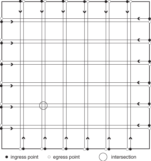
As in the previous models, the Manhattan mobility model introduced in Bai et al. (2003) also takes as input a map representing possible paths within the simulated region. As the name suggests, the map in the Manhattan mobility model is assumed to have the square block regular pattern typical of Manhattan-like models—see Figure 13.3. Each road in the Manhattan map has a single lane in each direction. Similar to the freeway mobility model, the path map implicitly defines ingress/egress points, and vehicles enter the simulated region from a randomly selected ingress point. However, once a vehicle has entered the simulated region, its trajectory is not deterministic as in the freeway mobility model; instead, its trajectory is essentially a Manhattan-like random walk: on reaching an intersection, a vehicle can proceed in the same direction with probability 0.5, or make a left or right turn with the same probability of 0.25. If a vehicle reaches the border of the simulated region, it can exit the region from one of the egress points.

Figure 13.3 Example map in the Manhattan mobility model.

The rules for setting a vehicle's speed are the same as those in the freeway mobility model: the velocity of a node at the next time step is dependent on its current velocity (the first rule in the freeway mobility model), provided it does not exceed the velocity of the preceding vehicle in the same lane if within the safety distance (the second rule in the freeway mobility model).

13.2 The SUMO Mobility Model

The models presented in the previous section only partially account for the distinguishing features of vehicular mobility described at the beginning of Chapter 12. In particular, while geographically constrained mobility is considered in all models, traffic rules and driver behavior are disregarded in the graph-based mobility model, while only a simple car-following rule is included in the freeway and Manhattan mobility models. Furthermore, other aspects of the mobility models described in the previous section can be considered as not accurately reflecting reality, such as the process of generating an individual trip, which is completely random and does not reflect traffic patterns observed in the real world. It is therefore clear that the models described above cannot be used to model vehicular mobility if the designer's goal is to gain an understanding of, say, vehicular networking protocol performance under realistic traffic conditions. To this end, a more accurate microscopic mobility model is needed, which is indeed able to reproduce vehicular traffic patterns observed in the real world. In turn, this requires on the one hand that the mobility model accounts for relatively complex traffic rules governing traffic lights and intersections, lane changing, lane merging, vehicle overtaking, etc., and, on the other hand, sophisticated tools should be provided to import and/or generate realistic road networks and traffic demand matrices.

A representative example of an advanced microscopic vehicular mobility model with these characteristics is the SUMO (Simulation of Urban MObility) mobility model (Team 2011a). SUMO was originally designed and is being maintained by members of the Institute of Transportation Research at the German Aerospace Center. SUMO is aimed at enabling relatively fast and accurate simulation of road networks comprising tens of thousands of edges—approximately corresponding to the size of a relatively large metropolitan area.

A notable feature of SUMO as compared to commercial microscopic models is that it is an open source model, thus it can be downloaded and installed for free (under a general public license) from the official SUMO homepage. This feature makes SUMO a very appealing choice for accurately modeling vehicular mobility, without the need to buy expensive commercial vehicular traffic simulators.

The main features of SUMO are summarized below:

The steps necessary for setting up a SUMO simulation are pictorially represented in Figure 13.4 and briefly described below:

Figure 13.4 Setting up a simulation with SUMO.

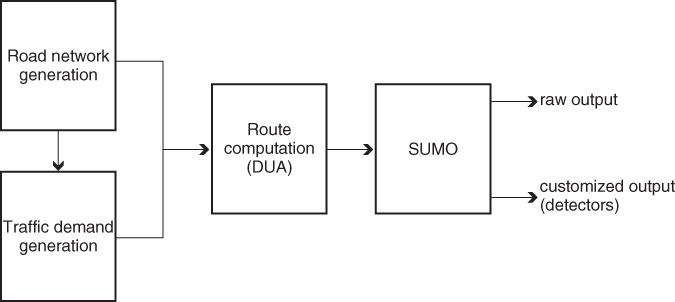
In the remainder of this section, we will describe in detail each of the SUMO building blocks shown in Figure 13.4.

13.2.1 Building the Road Network

SUMO provides two tools for building the road network: NETGEN and NETCONVERT. NETGEN is a road network generator, and allows three types of synthetic networks to be built: grid networks, spider networks, and random networks. Grid networks are Manhattan-like networks, where the user can decide on the number of intersections in the x- and y-axes, and the distance between intersections. Spider networks are defined by the number of axes dividing them, the number of concentric layers they are made of, and the distance between layers—see Figure 13.5 for an example of a spider network. Finally, random networks are randomly generated networks where certain parameters such as maximum and minimum road length, minimum angle between roads, etc., can be specified.

Figure 13.5 Example of spider road network with six axes and five concentric layers.

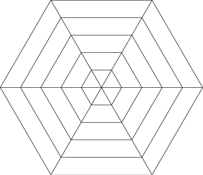
While synthetic road networks generated by NETGEN can be useful for an initial performance assessment, they are inadequate for accurately mimicking traffic patterns in a real-world situation. For this purpose, the NETCONVERT tool should be used instead. NETCONVERT allows both the definition of user-specified road networks—a tedious but sometimes unavoidable task—and importing existing road networks from several external sources such as VISUM, shape files, and digital map databases like OpenStreetMap. In the former case, an XML file called a SUMO network file can be defined to describe a digital road map. In the latter cases, NETCONVERT converts external digital maps into a native SUMO network file.

13.2.2 Building the Traffic Demand

There are different ways to build the traffic demand in SUMO. The most direct—but cumbersome—way is to define a route in the road network for each individual vehicle, including the trip starting time. Alternatively, traffic demands can be derived from user-defined flows and turning percentages at intersections. In turn, these values can be obtained from statistical data, traffic measurements, and so on. A third way of building the traffic demand is to generate routes between randomly selected origination and destination points, similar to what was done in the graph-based, freeway, and Manhattan mobility models. Finally, traffic demand values can be imported from existing data or from data generated by a macroscopic mobility model. These data can be expressed either in matrix form or as a trace of routes.

13.2.3 Route Computation

Once traffic demand is defined, routes can be computed. The basic approach for building routes is to use the Dijkstra shortest path algorithm to compute the shortest—or fastest, if speed limits are considered—route between each origin/destination pair. It should be noted, though, that due to traffic congestion, the best route as computed by the Dijkstra algorithm is not necessarily the one actually leading to the shortest possible travel time. In order to compute the best route considering also the effect of traffic congestion, which, in turn, depends on other vehicles' routing decisions, the Dijkstra algorithm must be iteratively executed several times, changing the weights on the edges of the road network reflecting the current vehicle's routing decisions at each iteration. This iterative process is terminated when equilibrium conditions are reached, corresponding to the best possible routes accounting also for traffic congestion. This more sophisticated approach to route computation is called dynamic user assignment and is an optional feature available in SUMO.

Static route computation is much faster than dynamic user assignment, and it is therefore suitable for simulating traffic in very large road networks where dynamic user assignment would be computationally too demanding. Static route computation is also the right choice for modeling situations in which a driver does not have a full view of the traffic situation in the area, and takes routing decisions based on stable information such as minimum distance to destination. On the other hand, dynamic user assignment is the right choice if the goal is to estimate, for example, the effects on traffic of introducing a new road in the network; in this case, it is useful to gain an understanding of the average travel time under the best possible conditions, namely, equilibrium conditions.

13.2.4 Running the Simulation and Generating Output

The final step is to run the simulation and generate output. Several models for traffic rules and driver behaviors are implemented in SUMO. In particular, SUMO defines rules for lane changing and lane merging, vehicle overtaking, car following, and sophisticated intersections for multi-lane roads. A driver behavioral model called the intelligent driver model (Treiber et al. 2000) is also implemented.

While the SUMO driving rules are designed to avoid accidents, these can be artificially created by requiring a vehicle to stop in the road for a sufficiently long time. As a consequence of accidents or other unexpected events, vehicle rerouting might be needed during the simulation. This can be done in SUMO by invoking the rerouter module, which changes a vehicle's route at run time.

During the simulation phase, several statistics of interest are collected by SUMO and returned as output of the simulation. These include vehicle-related data (e.g., a raw dump of a selected vehicle's position over time), road-related data (e.g., average flow traversing a certain road segment), trip-related data (e.g., average trip duration), and traffic light-based data (e.g., number of changes of each traffic light). Besides this standard output, personalized output can be obtained through the definition of detectors, which can be thought of as user-defined checkpoints in the road network where a certain quantity of interest can be tracked over time.

13.3 Integrating Vehicular Mobility and Wireless Network Simulation

We have so far described microscopic vehicular mobility models, highlighting their complexity if traffic rules and driver behavior are included in the model (cf. the SUMO model). However, what was described above represents only a part of the tasks to be accomplished if the goal of a network designer is to evaluate the performance of a vehicular network. In fact, a major difference between the simulation of other types of short-range wireless networks and the simulation of vehicular networks is that in most cases applications based on vehicular communications running onboard vehicles are expected, or even designed, to influence driver behavior.

Consider for instance the case of an active safety application such as the ones mentioned in Chapter 11—say, intersection collision warning (ICW). The purpose of such an application is to influence driver behavior, and in particular to allow the driver to reduce speed when approaching the intersection and come to a complete stop before it. In turn, changes in the mobility pattern of the warned vehicle will trigger similar changes in the mobility patterns of following vehicles. Hopefully, combinations of these modified mobility patterns will result in preventing a possible accident at the approaching intersection. Thus, the mobility pattern of vehicles should be modified on-the-fly in order to account for the effects of an ICW application running on the vehicular network. Another example of possible effects of vehicular network-based applications on mobility pattern is that of a smart navigation system, which exploits real-time information about traffic status gathered through the vehicular network to dynamically change the route to the destination in order to minimize travel time.

Note that the above situation—that is, applications that influence mobility patterns of the wireless nodes—is peculiar to vehicular networks: in all other application scenarios of short-range wireless networks considered in this book, with the partial exception of wireless sensor networks with intentional mobility, user applications running on the wireless nodes have no direct effect on a node's mobility pattern. Consider, for instance, a typical WLAN scenario. In this case, the user displays her/his own mobility patterns and is simply interested in staying connected to the network while moving.

What are the implications for the simulation procedure of the above observation about the intertwining between vehicular network applications and vehicle mobility patterns? The most important implication is that if accurate performance evaluation of vehicular network applications is sought, a close run-time interaction between the mobility and networking components of the simulator should be realized. In particular, it is not possible to feed the networking simulator with pre-computed mobility traces (as done extensively, for instance, in the simulation of opportunistic networks—see Part Six of this book).

Different architectural choices can be undertaken when designing a vehicular network simulator, which can be roughly divided into two categories. The first category comprises solutions in which the mobility and networking component of the simulator are closely integrated, essentially forming a single simulator. This is the case, for instance, for the vehicular network simulators presented in Harri et al. (2006) and Mangharam et al. (2005). Simulators in this class are typically realized by extending open source network simulators such as Ns2 with mobility models resembling vehicular mobility. However, due to the enormous challenges related to accurately modeling vehicular mobility as described earlier in this chapter, the mobility models integrated into the network simulator are typically relatively simple and inaccurate, thus impairing simulation accuracy. The alternative approach that has been pursued in the literature is to couple existing vehicular mobility and networking simulators by developing suitable tools/interfaces allowing the two simulators to interact with each other at run time. This is the approach undertaken, for instance, by Eichler et al. (2005), Lochert et al. (2005), and Wegener et al. (2008). The potential advantage of this approach is that both the mobility and networking component of the coupled simulator can be very accurate, if adequately chosen. On the other hand, simulation running time could become an issue.

In the remainder of this section, we will describe in detail a tool, called TraCI (Wegener et al. 2008), for coupling vehicular mobility and networking simulators. While in principle the tool could work in combination with arbitrary mobility and networking simulators, in the following we present its use with the SUMO vehicular mobility and Ns2 networking simulators, which are both relatively accurate and open source simulators.

13.3.1 The TraCI Interface for Coupled Vehicular Network Simulation

TraCI (Traffic ) is a tool for interlinking vehicular traffic and wireless networking simulators presented in Wegener et al. (2008). The main idea of TraCI is to run vehicular mobility and networking simulation in a stepwise fashion, alternating the simulation of a mobility step with that of a networking step, and having the outcome of each step given as input to the next step.

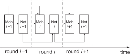
The stepwise approach to simulation realized through TraCI is pictorially represented in Figure 13.6. At each round, a mobility step is performed taking as input the outcome of the mobility step and the networking step in the previous round; the generated outcome is fed both to the networking step in the same round and to the mobility step in the next round. Similar to the mobility step, the networking step takes as input the outcome of the networking step in the previous round, and feeds the output to the mobility and networking step in the next round.

Figure 13.6 The TraCI stepwise simulation approach for coupling mobility and networking simulation.

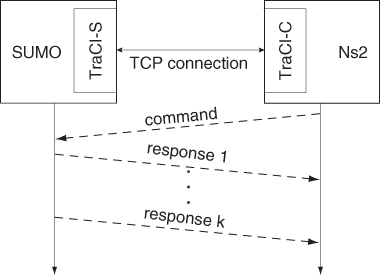
In order to realize the stepwise simulation approach described above, the authors extend SUMO and Ns2 so that they can interact according to the client–server paradigm through a Transmission Control Protocol (TCP) connection. More specifically, a TraCI-Server component is added to SUMO, and a TraCI-Client component is added to Ns2 (see Figure 13.7). The rationale for this choice is that the vehicular network application—which can potentially influence mobility patterns, as described above—runs in Ns2; hence, it is Ns2 that must be able to influence the SUMO simulation, which occurs through invocation of specific commands generated by the client application extending Ns2 and that are served by the server application extending SUMO.

Figure 13.7 The TraCI client–server architecture.

More specifically, the TraCI-Client can send the TraCI-Server a number of commands, which are grouped in three functional categories:

A number of response messages are sent back from the TraCI-Server to the TraCI-client in response to specific commands. These include:

• move node messages, reporting the status (position) of the nodes in the map;
• status messages, reporting to the client whether a certain command (e.g., change speed at a certain node) has been correctly executed.

For more details on TraCI and examples of its use, the reader is referred to Team (2011b).

References

Bai F, Sadagopan N and Helmy A 2003 IMPORTANT: A framework to systematically analyze the impact of mobility on performance of routing protocols for ad hoc networks. Proceedings of IEEE Infocom, pp. 825–835.

Baldessari R, Bodekker B, Deegener M, Festag A, Franz W, Kellum C, Kosch T, Kovacs A, Lenardi M, Menig C, Peichl T, Rockl M, Seeberger C, Strassberger M, Stratil H, Vogel H, Weyl B and Zhang W 2007 Car-2-Car Communication Consortium—manifesto (version 1.1). http://www.car-2-car.org/index.php?id-570.

Eichler S, Ostermaier B, Schroth C and Kosch T 2005 Simulation of car-to-car messaging: Analyzing the impact on road traffic. Proceedings of MASCOTS, pp. 507–510.

Harri J, Filali F, Bonnet C and Fiore M 2006 Vanet-MobiSim: Generating realistic mobility patterns for VANETs. Proceedings of ACM VANET (poster proceedings), pp. 96–97.

Lochert C, Caliskan M, Scheuermann B, Barthels A, Cervantes A and Mauve M 2005 Multiple simulator interlinking environment for IVC. Proceedings of ACM VANET (poster proceedings), pp. 87–88.

Mangharam R, Weller D, Stancil D, Rajkumar R and Parikh J 2005 GrooveSim: A topography-accurate simulator for geographic routing in vehicular networks. Proceedings of ACM VANET, pp. 59–68.

Team S 2011a SUMO—Simulation Of Urban Mobility. http://sumo.sourceforge.net/.

Team T 2011b Traffic Control Interface. http://sourceforge.net/apps/mediawiki/sumo/index.php?title = TraCI.

Tian J, Hahner J, Becker C, Stepanov I and Rothermel K 2002 Graph-based mobility model for mobile ad hoc network simulation. Proceedings of the ACM/IEEE Annual Simulation Symposium, pp. 337–344.

Treiber M, Hennecke A and Helbing D 2000 Congested traffic states in empirical observations and microscopic simulations. Physical Review E 62(2), 1805–1824.

Wegener A, Piòrkowski M, Raya M, Hellbruck H, Fischer S and Hubaux JP 2008 TraCI: An interface for coupling road traffic and network simulators. Proceedings of the ACM Communications and Networking SimulationSymposium (CNS), pp. 155–163.