
Chapter 15
Wireless Sensor Networks: Passive Mobility Models
As we saw in the previous chapter, WSNs find application in very diverse user scenarios. Although in many scenarios there is no mobility involved, applications of WSNs where mobility plays a role do exist. We can distinguish three different kinds of mobility in WSNs: (i) mobility of the sensor nodes; (ii) mobility of the sink node(s); and (iii) mobility of a monitored event/object. The first kind of mobility occurs when at least part of the sensor nodes is mobile. Examples of sensor node mobility are when sensor nodes are dispersed and free to move in the monitored region (e.g., sensor nodes floating on the surface of the ocean), or when they are installed on animals for wildlife tracking and monitoring. The second kind of mobility refers to a situation in which sink nodes are able to autonomously move in the monitored region, with the purpose of collecting data from the sensor network. Finally, the third kind of mobility occurs when a WSN is used for monitoring or tracking purposes, and works under the event-driven data model. In this case, modeling the occurrence and mobility of an event to be monitored (e.g., a gas leak and movement of the resulting gas plume) is useful for understanding the resulting data traffic pattern in the WSN. Similarly, when the WSN is used for target tracking, modeling target movement is useful for estimating the amount and pattern of data generated in the WSN during target tracking.
These types of WSN mobility typically occur in isolation: that is, if sensor nodes are mobile because, say, they are floating on the surface of the ocean, sink nodes are typically fixed—they are, for instance, installed on buoys. On the other hand, when mobile sink nodes are used to gather data collected by a WSN, the sensor nodes comprising the WSN typically are fixed, and so on. Cases in which at least two of the three types of WSN mobility coexist are relatively scarce, although possible.
Independently of whether mobility occurs in the sensor nodes, in the sink nodes, or in the target/monitored event, we can distinguish two radically different forms of mobility in WSNs: passive and active mobility. In the former case, mobile entities are not capable of performing autonomous movements, and their mobility is caused by some external force, such as animal movements, wind, ocean flows, and so on. In the latter case, mobile entities are instead capable of performing autonomous movements, that is, they can decide when to move and stop, and the destination/trajectory of their movements. In this chapter, we will present representative models of passive mobility in WSNs, while the next chapter will be devoted to active mobility models.
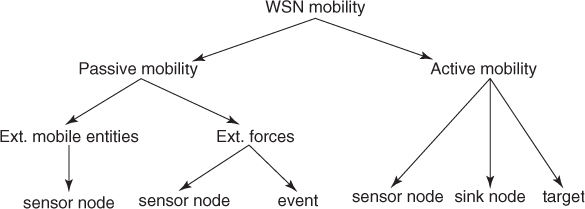
A taxonomy of mobility models for WSNs is displayed in Figure 15.1. Mobility can be either passive or active. Passive mobility can be caused either by mobility of the entity to which a sensor node is attached, or by external forces. Passive mobility caused by external forces can model movement both of sensor nodes and of a natural event to be monitored. Active mobility can refer to active mobility of sensor nodes, of sink nodes, or of a target being tracked by the WSN—see next chapter.
Figure 15.1 A taxonomy of mobility models for WSNs.
15.1 Passive Mobility in WSNs
As mentioned above, passive mobility in WSNs occurs when the mobile entities are not capable of performing autonomous movements, but move in response to external forces. Two main classes of passive mobility are present in WSNs, both of them referring to the case in which sensor nodes are mobile. The first class is when sensor nodes are installed on mobile entities (e.g., people, animals, moving vehicles, etc.), in which case the mobility of sensor nodes becomes equivalent to the mobility of the entity carrying the sensor node. The second class of passive mobility encompasses situations in which sensor nodes are not fixed, but are free to move in the environment in response to some external force such as wind, ocean flows, and so on. In this case, mobility of sensor nodes can be modeled through modeling the external force and the effects of this force on a sensor node. Models of natural forces can also be used to estimate the movement of an event (say, a gas plume) monitored by a WSN.
In the remainder of this chapter, we will present representative models for both classes of passive mobility: in the next section we will describe two mobility models for wildlife tracking applications, while in Section 15.3 we will describe a mobility model aimed at modeling the dispersion of sensor nodes floating in a large body of water.
15.2 Mobility Models for Wildlife Tracking Applications
In this section, we present two mobility models for applications of WSNs to wildlife tracking scenarios. In these scenarios, sensor nodes are installed on animals, so mobility models for this class of applications aim at closely resembling animal movements. The first is the model introduced in Juang et al. (2002) as an outcome of the ZebraNet project (Martonosi et al. 2004). The second model was introduced in Small and Haas (2003) to resemble movements of a population of whales.
Besides using more specific mobility models such as the ones described below, simpler general-purpose mobility models could be used as well in wildlife tracking applications, at least for the purpose of gaining a first understanding of WSN performance. In particular, the Lévy flight model described in Section 4.2.2, which, we recall, is a random walk-like model in which erratic behavior in a close neighborhood is occasionally complemented with long-distance travel, has been shown in the literature to resemble animal movement quite accurately.
15.2.1 The ZebraNet Mobility Model
The ZebraNet mobility model was derived in Juang et al. (2002) as an outcome of the ZebraNet project, whose purpose was the fine-grain monitoring of movements of a population of zebras in the Laikipia ecosystem of central Kenya. A first observation made in the ZebraNet project was that, due to the features of the zebra social system as observed by zoologists, installing sensor nodes on selected male individuals was sufficient to monitor movements of a much larger population of zebras. In fact, zebras are organized in so-called “harems,” formed of a single adult male zebra, 4–5 females, and their young offspring. Although females typically initiate movements, the males often adjust the direction and speed of movement of the group. Thus, installing a single sensor node on an adult male zebra is sufficient for fine-grained tracking of a group of about 10–12 zebras.
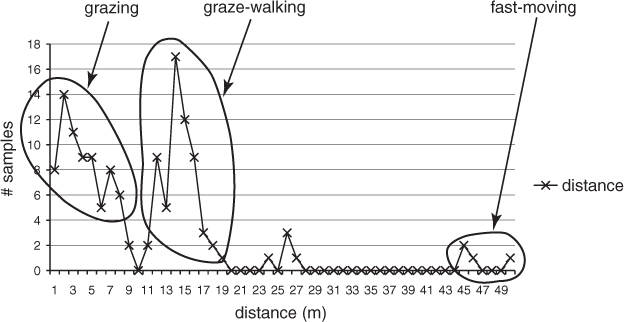
Zebra movement patterns can be characterized in terms of three main states: grazing, graze–walking, and fast-moving. Zebras spend most of their time in a grazing state, during which mobility is characterized by low movement rates and high turning angles. In the graze–walking state, zebras walk deliberately, with heads lowered, and clip vegetation as they move. Mobility in this state is characterized by higher movement rates and smaller turning angles than those displayed in the grazing state. Finally, zebras occasionally move much more quickly (fast-moving state), usually because of the presence of predators, or because an area's vegetation has been exhausted. Mobility in this state is characterized by high movement rates and small turning angles.
Besides the three-state behavior, another characterizing feature of zebra mobility is that zebras look for water about once per day. When they reach a water source, they remain there for a relatively short time, after which they start behaving normally (alternating between grazing, graze–walking, and fast-moving states) until the next day. Finally, zebras tend not to have long periods of motionless sleep, due to the need to keep watch and avoid predators. Hence, the mobility pattern described above applies 24 hours a day.
In order to monitor zebra movements, the following parameters were tracked in the ZebraNet project with a periodicity of three minutes, which is considered by zoologists as an optimal time interval for sampling animal movements (Altmann 1974): the movement distance and the turning angle. The movement distance is defined as the net distance between the position of the zebra at the beginning and end of a three-minute interval. Similarly, the turning angle is defined as the absolute value of the angle between the position of the zebra at the beginning and end of a three-minute interval.
The distribution of observed movement distances is shown in Figure 15.2. The three movement statuses can be identified quite well in the distance distribution, which appears to be bimodal. In the first mode—grazing—the mean net distance is 3.1 m, with a peak at 2 m; in the second mode—graze–walking—the mean net distance is 13 m with a peak at 14 m. Finally, the few outliers at the tail of the distribution correspond to the fast-moving status.
Figure 15.2 Distribution of movement distances covered by zebras.
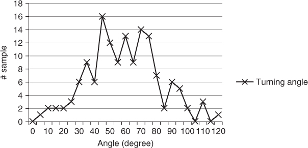
The distribution of observed turning angles is shown in Figure 15.3. Different from the movement distribution, the turning angle distribution does not present a shape allowing a clear distinction of the mobility states. In general, we can observe that most observed angles lie in the 30–90 degree interval, with a peak at 45 degrees.
Figure 15.3 Distribution of zebra turning angles.
Based on the above observations, Juang et al. (2002) define the following model to resemble the mobility of zebras. The mobility region is a square area of 20 × 20 km, approximately corresponding to the area of the Laikipia ecosystem. At the beginning of the simulation, 20 water sources are randomly located in the area, as well as 50 zebras. After initial deployment, each zebra (assumed to be the leading male of a group) starts moving independently of the others, according to the empirically derived distance and turning angle distributions shown in Figures 15.2 and 15.3. Zebras move at a base speed of 0.017 m/s while grazing, four times faster at 0.0723 m/s when graze–walking, and nine times faster at 0.155 m/s while fast-moving. Once per day, each simulated zebra becomes thirsty. When thirsty, the zebra moves into the graze–walking state and starts moving toward the closest water source.
15.2.2 The Whale Mobility Model
The whale mobility model was introduced in Small and Haas (2003) to model movement of radio-equipped whales. The idea of Small and Haas (2003) is to replace current whale tracking systems based on frequent offload of tracked data from single whales through satellite communications with a lower cost alternative based on WSNs. Their idea is to deploy a number of sink nodes in selected feeding grounds where whales are known to periodically return, and to gather data from whales through high data rate (compared to satellite communications) wireless links established between radio-equipped whales and sink nodes. Furthermore, collected data can be exchanged between whales when within each other's transmission range, thus allowing multi-hop data propagation to reach a sink node. Since whales are expected to come into contact with a sink node or another whale periodically, a relatively large amount of memory to store data needs to be installed on the sensor nodes deployed on whales. However, the higher costs induced by these higher memory needs are more than compensated by the reduced cost of the communication infrastructure.
In order to model mobility of whales in this application scenario, Small and Haas (2003) start from some observations made by biologists. In particular, it has been observed that whale movement is influenced by three main factors: migration, grouping with other whales, and direction of the nearest feeding grounds. Thus, mobility of whales in Small and Haas (2003) is modeled as the result of a sum of three suitably weighted vectors, representing the contribution to movement of migration, grouping, and feeding, respectively. More specifically, the weighted vector sum is used to determine the movement direction, while movement speed is selected according to the following rules: the speed of a whale is randomly chosen between vmin = 2 m/s and vmax = 3 m/s for whales outside the feeding grounds, and between vmin = 0 m/s and vmax = 1 m/s when within the feeding grounds. The movement status of each whale is updated every time step t, upon which new speed and direction values are generated for the next time step.
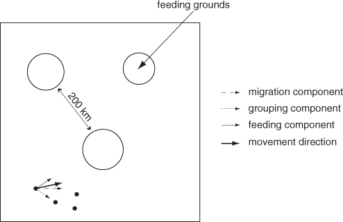
As mentioned above, direction of movement is computed as the weighted sum of three components. The first component is determined by the migration pattern. A migration direction is determined for each whale, which is defined as a preferred movement angle rather than an absolute direction. More specifically, the migration direction is expressed as the mean of a Gaussian distribution representing the migration angle. At each time step, a whale is assigned with a new migration direction randomly generated according to the Gaussian migration angle distribution, with a predetermined standard deviation. The role of the standard deviation in the migration pattern is quite evident: a larger standard deviation results in a more random migration pattern. The weight of the migration component of movement direction is fixed at 1.
The grouping component of movement direction is computed as follows. When a whale comes within a certain fixed range of other whales, it sets its grouping directional component in the direction of the closest female. When a whale becomes part of a group, its mobility is governed by the same migration and feeding behaviors of the other members of the group. The weight of the grouping direction is a Gaussian random variable, with the mean set to 0.8 and standard deviation set to 0.5. In order to allow whales to leave a group, a maxGroupingTime variable is introduced in the model, which is set to 3 in Small and Haas (2003). If the whales have grouped for longer than maxGroupingTime, then the weight of the grouping component of movement direction is set to 0 in the next time step.
The feeding component of the movement direction is generated as follows. First of all, a number of feeding grounds modeled as circular regions with a random radius between 20 and 30 km are generated in the movement region. Feeding grounds are assumed to be separated by a distance of about 200 km. The direction of the feeding component of the movement corresponds to the direction pointing to the closest feeding ground. The weight of the component is computed according to a variable hungry, modeling a whale's feeling of hunger. The variable is increased when the whale is swimming outside the feeding grounds, and decreased when it is swimming inside the feeding grounds. The weighting factor of the feeding component is computed according to a Gaussian distribution with mean 0.4 · hungry and standard deviation 0.3 · hungry.
After the weighted sum of the three directional components has been computed, a motion consistency factor is introduced, in order to avoid motion patterns in which whales completely change direction at each time step. This factor takes values in the [0, 1] interval. Denoting by θi the direction at time step i, we have that the new direction θi+1 at time step i + 1 is computed as follows:
![]()
where cf ∈ [0, 1] is the consistency factor, and ![]() is the direction for time step i + 1 as computed by the weighted directional sum described above. A pictorial view of the whale mobility model is shown in Figure 15.4.
is the direction for time step i + 1 as computed by the weighted directional sum described above. A pictorial view of the whale mobility model is shown in Figure 15.4.
15.3 Modeling Movement Caused by External Forces
In some application scenarios, movement of sensor nodes, or of a monitored event, can be caused by external natural forces, such as wind, ocean flows, and so on. In such cases, mobility models can be derived from models used to describe the natural phenomena exerting the force. In this section, we present one of the few mobility models for WSNs aimed at modeling the effect of a natural force on sensor nodes. The model was introduced in Caruso et al. (2008) to model the effect of ocean flows on underwater mobile sensor networks, and is called the meandering current mobility model.
Figure 15.4 Pictorial view of the whale mobility model.
The application scenario considered in Caruso et al. (2008) is an underwater sensor network in which a number of floating or drifting sensor nodes are released underwater in a relatively small area, and are then left free to move with the underwater ocean flows. Sensor nodes are able to communicate with each other, if close enough, through acoustic wireless links. The purpose of the sensor network is to monitor the ocean currents and underwater habitat.
Caruso et al. (2008) exploit a physically inspired model of ocean flows to model mobility of floating/drifting sensor nodes. Definition of the model starts from the observation that oceans are a stratified, rotating fluid, hence vertical movements, although occasionally present, are negligible with respect to the horizontal ones. Thus, sensor nodes can be assumed to move over a two-dimensional horizontal surface, instead of in a three-dimensional volume. The goal of the model is to describe movement of sensors for a relatively long period of time (several days) in a relatively large region, spanning several kilometers.
An incompressible, two-dimensional flow can be described by a suitably defined stream function ψ = ψ(x, y, t), from which the velocity components in x and y coordinates can be derived as follows:
![]()
where u is the eastward component and v is the northward component of the velocity field. Then, the trajectory of a device floating in the flow can be computed as the solution of the following system of ordinary differential equations:
![]()
So, the trajectory of a floating device can be readily computed once the stream function describing the behavior of the flow is defined. Caruso et al. (2008) use a widely studied stream function first defined in Bower (1991) and later generalized by Samelson (1992), which has been designed to capture the main features of a typical ocean flow, namely, currents and vortices. The stream function, known as the meandering jet model since it represents a jet-like current meandering between recirculating vortices (see Figure 15.5), is defined as follows:
where B(t) = A + ϵcos(ωt), k is a parameter corresponding to the number of meanders per unit length, c is the phase speed with which they shift downstream, and B is a time-dependent function modulating the width of the meanders; parameter A determines the average meander width, ϵ is the amplitude of the modulation, and ω is its frequency.
Figure 15.5 Jet-like current meandering between recirculating vortices.
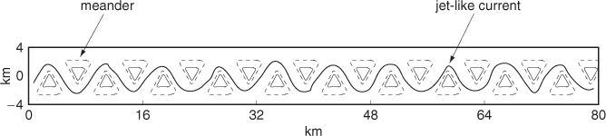
Caruso et al. (2008) suggest using the meandering jet model with the following parameters: A = 1.2, c = 0.12, k = 2π/7.5, ω = 0.4, and ϵ = 0.3. With these parameters, and by setting the length and time unit to 1 km and 0.03 days, respectively, we have that the average size of meanders is about 7.5 km, the peak speed inside the jet is about 0.3 m/s, and the modulation period is about half a day (corresponding to the main tidal period).
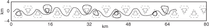
The motion patterns of a group of 30 sensor nodes initially deployed in a 4 × 4 km area are shown in Figure 15.6. As can be seen from the figure, the sensor nodes are initially very close to each other, but, as time goes by, they become more and more dispersed along the flow; after three days, the distance between the eastern and western sensor node in the flow is more than 60 km. Figure 15.7 shows a typical sensor path, with an alternation between phases of fast downstream motion when the sensor node is in the jet current, and looping motion when the sensor node is captured in a vortex. Notice that sensor node trajectories are highly correlated when they are trapped in the same vortex, while they are almost independent when they travel in the jet stream.
Figure 15.6 Motion patterns of a group of 30 sensor nodes initially deployed in a square of side 4 km.
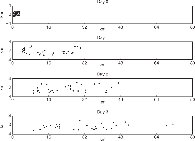
Figure 15.7 Trajectory of a typical sensor node path in the meandering current mobility model.
Altmann J 1974 Observational study of behavior: Sampling methods. Behavior 49, 227–267.
Bower A 1991 A simple kinematic mechanism for mixing fluid parcels across a meandering jet. Journal of Physical Oceanography 21(1), 173–180.
Caruso A, Paparella F, Vieira L, Erol M and Gerla M 2008 The meandering current mobility model and its impact on underwater mobile sensor networks. Proceedings of IEEE Infocom, pp. 771–779.
Juang P, Oki H, Wang Y, Martonosi M, Peh LS and Rubenstein D 2002 Energy-efficient computing for wildlife tracking: Design tradeoffs and early experiences with ZebraNet. Proceedings of ACM ASPLOS, pp. 96–107.
Martonosi M, Lyon S, Peh LS, Poor V, Rubenstein D, Sadler C, Juang P, Liu T, Wang Y and Zhang P 2004 http://www.princeton.edu/mrm/zebranet.html.
Samelson R 1992 Fluid exchange across a meandering jet. Journal of Physical Oceanography 22(4), 431–440.
Small T and Haas Z 2003 The shared wireless infostation model - a new ad hoc networking paradigm (or where there is a whale, there is a way). Proceedings of ACM MobiHoc, pp. 233–244.