
Chapter 18
Routing in Opportunistic Networks
In the previous chapter, we described the distinguishing features of opportunistic networks, namely, sparse node density, lack of network-wide connectivity, and unique role of node mobility as communication means within the network. Given these features, the mechanisms governing message routing in an opportunistic network are very different from those typical of other types of wireless networks. In particular, lack of end-to-end communication paths between source and destination of a message forces the routing protocol to exploit the temporal dimension and node mobility to eventually deliver a message to the intended destination.
In this chapter, we will first describe the basic store, carry, and forward mechanism at the heart of any opportunistic network routing protocol, and present a few representative routing protocols for opportunistic networks. We will then carefully discuss the role of mobility in message routing, and define the most important mobility metrics used in the characterization and analysis of node mobility in opportunistic networks.
18.1 Mobility-Assisted Routing in Opportunistic Networks
Given the lack of end-to-end communication paths between source and destination of a message, the mechanisms at the basis of routing in opportunistic networks are radically different from those used in other types of wireless networks, such as route discovery/route reply messages, routing tables, and so on. In opportunistic networks, routing protocols are based on the store, carry, and forward principle, according to which a message M generated by a source node S is stored in S's buffer and carried around, until a communication opportunity for node S with another node A arises. At that point, M can be forwarded to node A, either transferring or duplicating M into its buffer. This message propagation process is repeated until, at some point in time, a node carrying a copy of M in its buffer gets in touch with the destination node D, at which point the delivery of M to the destination takes place.
Although based on the same principle, routing protocols for opportunistic networks differ considerably due to the different design choices concerning: (i) the number of copies of a message circulating in the network; and (ii) the amount/type of network state information used by nodes to drive the message-forwarding process.
As regards the number of copies, routing protocols proposed in the literature can be classified into single-copy and multi-copy protocols. In the former case, only a single copy of the message is allowed to be present in the network at any point in time. The message is originally held by the source node S, which might either keep it till it directly gets in touch with the destination node, or decide to hand M to another node A. Decisions on whether to hand the message to another node are typically driven by metrics aimed at measuring the likelihood of a node to meet the destination node. While single-copy approaches induce minimal load in the network due to the lack of message replication, they typically fall short in terms of message delivery delay and successful message delivery rate, unless the mobility pattern of nodes is very predictable.
Multi-copy protocols have been introduced with the purpose of reducing delay and increasing success rate in delivering messages, at the expense of increasing message overhead. Multi-copy protocols allow replication of a message when communication opportunities arise. These protocols can be further divided into controlled and uncontrolled multi-copy approaches, depending on whether the message replication process is controlled or not. Control of the replication process is typically realized by either imposing a strict upper bound L on the number of copies of the message M circulating in the network, or putting an upper bound on the number of hops that a message can travel on its way to the destination, or both. While in uncontrolled multi-copy protocols the message overhead cannot be directly kept under control, in controlled approaches the tradeoff between delivery delay/success rate and message overhead can be carefully tuned. Note also that single-copy protocols can be considered as an instance of controlled multi-copy protocols if the upper bound L on the number of message copies is set to 1.
Besides the number of copies of a message circulating in the network, the other major design choice in opportunistic routing protocols concerns the way that forwarding decisions are taken when a communication opportunity arises. Suppose a node A currently holding a copy of M meets another node B, and that, given the rules on the number of M copies, A could potentially replicate M into B's buffer. What rule is used to decide whether to replicate M or not? In other words, what is node A's forwarding strategy? Note that this question is relevant only for single-copy or controlled multi-copy approaches, since in the case of uncontrolled multi-copy approaches M is always duplicated into node B's buffer.
Forwarding strategies presented in the literature can be divided into two broad classes, depending on whether or not they make use of network state (also known as context) information to undertake forwarding decisions. In the former class of strategies, the forwarding choice is based on a set of metrics aimed at predicting node B's likelihood of meeting the destination. These metrics are based on some network state information locally available at the node, which, depending on the specific routing protocol, can take the form of history of past encounters, profiles of recently encountered nodes, storage of a portion of a social graph, and so on. In the latter case, the forwarding strategy is very simple, and states that M is always duplicated into B's buffer provided rules on the number of message copies circulating in the network and/or number of hops are not violated. Clearly, network state-based protocols tend to have superior performance to network-oblivious protocols, since forwarding decisions are based on a richer amount of information. However, locally storing a portion of the network state on the nodes comes at a cost in terms of storage resources, which are used to store state information instead of additional network messages. Hence, whether network state-based approaches are superior to network-oblivious ones in the presence of limited storage capacity depends on the considered application scenario and on the node mobility pattern.
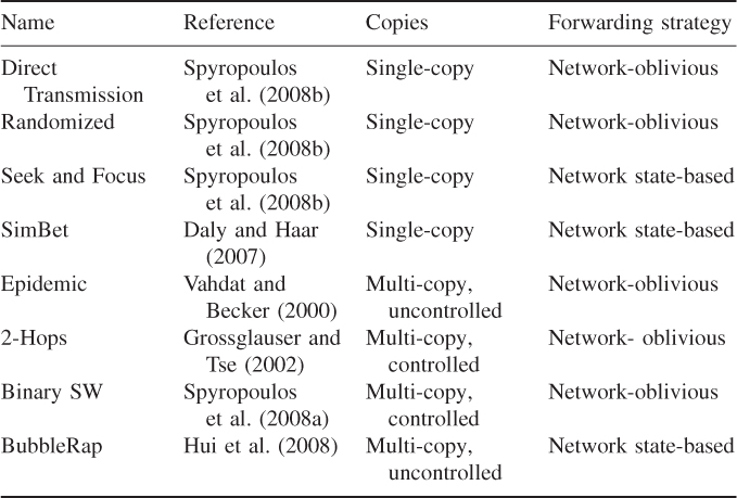
Table 18.1 presents a number of representative routing protocols for opportunistic networks, and their classification according to the criteria described above. In the rest of this section, we will describe in detail a few protocols belonging to different classes, focusing our attention mostly on network-oblivious routing protocols, whose performance is much easier to analyze formally. In fact, formal analysis of network state-based protocols would require accounting for the evolution of locally available network state information on the nodes, which contributes to making the analysis very complex.
Table 18.1 Some representative routing protocols for opportunistic networks
18.1.1 Single-Copy Protocols
The simplest possible single-copy routing protocol is Direct Transmission (see, e.g., Spyropoulos et al. (2008b)), according to which the source node S keeps the single copy of M in its buffer until either M's time-to-live (TTL) counter expires, or S gets in touch directly with the destination D and delivers the message. Direct Transmission minimizes communication overhead—at most, a single transmission between S and D is performed—at the expense of very long average message delivery delays and low message delivery ratios. Clearly, the performance of Direct Transmission depends on the node mobility pattern: if S and D meet each other relatively frequently, the delay and message delivery ratio can be satisfactory also with this simple routing protocol; however, in most cases Direct Transmission provides poor performance.
A less trivial example of a single-copy routing protocol is the Seek and Focus protocol proposed in Spyropoulos et al. (2008b). The protocol builds upon knowledge of network state locally stored at the nodes. More specifically, every node in the network is assumed to store a timer for every other node in the network, recording the time elapsed since the two nodes last encountered each other. Encounter timers are used by nodes to locally compute a utility function according to the following rules: let Ui() be the utility function for node i; for each j ≠ i, Ui(j) is an arbitrary monotonically decreasing function of the encounter timer τi(j) between nodes i and j, satisfying the property that ![]() .
.
The Seek and Focus protocol is a hybrid approach which alternates between randomized and utility-based forwarding. More specifically, the protocol alternates the following phases. In what follows, Uf denotes a predefined utility threshold, 0 < p < 1 a predefined forwarding probability, and δ a predefined forwarding threshold.
Another interesting single-copy routing protocol is SimBet (Daly and Haar 2007), which attempts to exploit information related to the social relationships between network members to optimize the forwarding process. SimBet exploits two metrics to predict the likelihood of a node meeting the destination: similarity and betweenness. Similarity measures the number of common neighbors between two network nodes: denoting by LA and LB the list of nodes encountered by nodes A and B, respectively, the similarity between A and B is the number of nodes occurring in both lists, that is, ![]() . Betweenness instead is a centrality metric aimed at measuring how well a node can facilitate communication to other nodes in the network—see the next chapter for a formal definition of centrality metrics. Note that both similarity and a version of the betweenness metrics computed on a local view of the network can be computed locally when two nodes meet each other if the two nodes exchange their contact lists. The similarity and betweenness metrics are used to compute a utility value in the [0, 1] interval, with higher utility values indicating a relatively higher likelihood of meeting the destination node. The utility metric is then used to drive the forwarding process: if node A holding message M destined for node D meets another node B, it hands over M to B only in case B has a higher utility (computed with respect to node D) than node A.
. Betweenness instead is a centrality metric aimed at measuring how well a node can facilitate communication to other nodes in the network—see the next chapter for a formal definition of centrality metrics. Note that both similarity and a version of the betweenness metrics computed on a local view of the network can be computed locally when two nodes meet each other if the two nodes exchange their contact lists. The similarity and betweenness metrics are used to compute a utility value in the [0, 1] interval, with higher utility values indicating a relatively higher likelihood of meeting the destination node. The utility metric is then used to drive the forwarding process: if node A holding message M destined for node D meets another node B, it hands over M to B only in case B has a higher utility (computed with respect to node D) than node A.
18.1.2 Multi-Copy Protocols
The simplest possible multi-copy routing protocol is Epidemic (Vahdat and Becker 2000) which, as the name suggests, resembles an epidemic spreading disease in a population. In Epidemic routing, initially only the source node S holds a copy of M and it is thus infected. Whenever an infected node A (i.e., a node holding a copy of M in its buffer) meets a non-infected node B, the infected node makes a duplicate of message M and copies it into the buffer of the non-infected node, thus making it infected.
Despite its simplicity, Epidemic routing is widely considered in opportunistic network performance evaluation. In fact, it has been shown that, as intuition suggests, Epidemic routing provides minimum message delivery delay if the buffer size on the nodes is assumed to be infinite. On the other hand, it is well known that Epidemic routing performance quickly degrades if node buffers have limited size: this is due to the very large message overhead induced by Epidemic routing, which quickly overloads node buffers leading to message losses.
Several controlled multi-copy routing protocols have been introduced in the literature with the purpose of reducing message overhead while at the same time providing acceptable performance in terms of message delivery delay.
A first example of this class of protocols is 2-Hops routing (Grossglauser and Tse 2002; Spyropoulos et al. 2008a). In 2-Hops routing, the source node S holds L ≥ 1 copies of the message M. Node S delivers a single copy of M to the first L − 1 nodes encountered—which become relay nodes—and keeps the last copy of the message for itself. Relay nodes are not allowed to forward their copy of M to other nodes, but they can deliver it only to the destination. Thus, the message is eventually delivered to the destination by either S, or one of the (up to) L − 1 relay nodes.
2-Hops routing controls both the number of message copies circulating in the network (L at most) and the number of hops in the source/destination path. In fact, since relay nodes can only deliver the message to the destination, the maximum length of the source/destination path is two hops, whence the name of this protocol.
Binary Spray and Wait (SW) (Spyropoulos et al. 2008a) can be regarded as an optimization of 2-Hops routing. In Binary SW, L is assumed to be a power of 2. Initially, the source node S holds all the L = 2q copies of the message. When a node with h ≥ 2 copies of the message meets a node without message M, it hands the new node h/2 of its copies, and keeps the other h/2 for itself. When a node remains with a single copy of M, it can deliver this single copy only to the destination node. It is easy to see that the number of hops in the source/destination path is upper bounded also in Binary SW, and the upper bound is q = log2L.
All the protocols described so far make no use of network state information. Several protocols have been proposed that exploit some form of locally stored network state information to optimize the message-forwarding process. Of particular interest in this class of protocols are those exploiting information about the social structure underlying the opportunistic network to optimize performance.
A representative example of this class of protocols is BubbleRap (Hui et al. 2008). BubbleRap builds upon two assumptions: (i) nodes are divided into communities, possibly overlapped, and possibly composed of a single node; and (ii) each node has a global ranking—computed through a centrality metric such as betweenness—across the whole network, as well as a local ranking within its local community(ies). Intuitively speaking, message routing is a hierarchical process performed as follows: when node S wants to send a message M to node D, it first attempts to bubble the message up the hierarchical ranking tree using the global ranking value, with the goal of delivering M to socially “well-connected” nodes. This process is repeated until a node B belonging to the same community as the destination is reached. Starting from this point, the local ranking value of the destination community is used to drive the routing process to the destination node. In order to reduce the message overhead, a heuristic is implemented requiring the original carrier of a message to delete M from its buffer when the message is delivered to a node in the destination community.
18.2 Opportunistic Network Mobility Metrics
We have seen in the previous section that mobility plays a fundamental role in the process of delivering a message from source to destination. It is then clear that mobility modeling on the one hand, and analysis of mobility properties observed in real-world traces on the other hand, have attracted considerable attention in the opportunistic networking community. In particular, a number of metrics related to node mobility have been defined and utilized in the literature to analyze the performance of opportunistic network routing protocols.
18.2.1 The Expected Meeting Time
A first important mobility metric is the expected meeting time (EMT), which is formally defined as follows.
It is well known that some mobility models, such as RWP, give rise to a non-uniform node spatial distribution in stationary conditions. This is why, in the definition of EMT, it is required that nodes A and B are initially distributed according to the stationary node spatial distribution of the mobility model at hand.
EMT is especially important in characterizing the performance of network-oblivious routing protocols. In fact, in this class of protocols, a message held by node A is either forwarded to another node B upon their first encounter, or is not forwarded to B at all—for instance, because the upper bound L on the number of message copies and/or the upper bound on the number of hops has been reached. Thus, taking as t = 0 the instant of time when node A gets a copy of M, EMT is a good estimate of the time when node A is expected to encounter node B for the first time.
EMT for some well-known geometric mobility models has been derived by Spyropoulos et al. (2006). For instance, EMT in the presence of RWP mobility has been shown to be as follows:
![]()
where A(R) is the area of the mobility region R, r is the transmission range, ![]() is the expected length of a trip,
is the expected length of a trip, ![]() is the expected duration of a trip,
is the expected duration of a trip, ![]() is the expected pause time at waypoints, and
is the expected pause time at waypoints, and ![]() ) is the probability that a node is moving at any time.
) is the probability that a node is moving at any time.
Note that the above expression can be significantly simplified in case the pause time is set to 0. In fact, in this case we have ![]() , from which we can write
, from which we can write
![]()
where ![]() is the expected speed in a trip.
is the expected speed in a trip.
A metric closely related to the meeting time is the hitting time, defined as the time needed for a node to move into the transmission range of a fixed, randomly chosen point in the movement region R, starting from the stationary node spatial distribution of ![]() . The hitting time for some well-known geometric mobility models has been derived in Spyropoulos et al. (2006).
. The hitting time for some well-known geometric mobility models has been derived in Spyropoulos et al. (2006).
18.2.2 The Inter-Meeting Time
Another metric that has been thoroughly studied in the opportunistic networking literature is the inter-meeting time—also called inter-contact time—which, informally speaking, is intended to measure the time elapsing between two consecutive meetings of the same pair of nodes. The inter-meeting time is important for studying the performance of network state-based routing protocols, since it can be used to estimate the time elapsing between successive communication opportunities of a node pair. Estimating this quantity is important in the evaluation of network state-based routing protocols, where a copy of message M is not necessarily forwarded from node A to B upon their first encounter after M has reached A—for instance, because the local view of the network state stored at A and/or B has changed in the time elapsing between the first and the second communication opportunity.
In the literature, two different definitions of the inter-meeting time can be found, which we report for completeness. In Groenevelt et al. (2005), the inter-meeting time is defined as the time elapsing between the starting time of two consecutive meetings of a node pair, where a meeting between nodes A and B is defined as a continuous-time interval during which nodes A and B are within each other's transmission range. Formally:
The other definition of inter-meeting time, used for instance in Cai and Eun (2009) and Karagiannis et al. (2007), and more commonly used in the literature, defines the inter-meeting time as the time elapsing between the ending time of a meeting and the starting time of the next one. Formally:
The inter-meeting time has been studied for synthetic mobility models, as well as estimated from observations made in real-world experiments. In the next chapter we will report extensively on existing studies of inter-meeting time characterization based on real-world data traces. As for the inter-meeting time in synthetic mobility models, it has been formally proven in Cai and Eun (2009) that well-known mobility models such as RWP and RW give rise to an inter-meeting time distribution whose tail decays at least exponentially with time.
18.2.3 Contact Duration
The third metric which is typically considered in opportunistic network performance evaluation is contact duration, which can be informally intended as the expected duration of a meeting between any two nodes A and B. Formally, contact duration is defined as follows:
The metric defined above becomes relevant when the expected time needed to transfer the message M from A to B is very large—say, several seconds or minutes. Typically, this happens when M is a multimedia file such as a picture or a video. In these situations, it is very likely that the contact duration is not long enough to ensure complete transfer of M from A to B.
In general, estimating contact duration is necessary for understanding whether situations of incomplete message transfer between nodes such as the one described above are likely to happen. If, for instance, the contact duration is estimated to be in the range of 1–2 minutes and the average size of M is 1 MB, a few seconds are sufficient to transmit M from A to B even with the relatively slow Bluetooth technology; hence, it can be concluded that the event “message transfer between A and B during a contact is interrupted” is relatively unlikely. Under this assumption, contact opportunities between nodes can be well approximated by instantaneous “contact” events during which message M is entirely transferred, and the actual duration of the contact becomes irrelevant. On the other hand, if the expected message transfer time is comparable to the expected contact duration, the above simplifying assumption cannot be made, and the analysis of the message propagation process within the network becomes more complex.
A possible solution to avoid incomplete message transfer during a contact is to break down a relatively large message M into smaller pieces M1, …, MK, and to transfer as many pieces as possible to the other node during a contact. This approach can be combined with network coding techniques to improve message delivery performance.
18.2.4 Relating the Three Metrics
The three mobility metrics defined above are clearly related to each other, as depicted in Figure 18.1. The difference between EMT and the inter-meeting time lies in the starting time of the observation interval: in the case of inter-meeting time, the observation of mobile nodes A and B starts at the moment when a contact between A and B has just ended. Thus, observation of A and B is done conditional on the knowledge of a recently past event, namely, a contact between A and B. On the contrary, in case of EMT no assumption on past contact between nodes is made, and the observation is assumed to start at a random point in time—that is, the observation is not conditioned on any past event. Note that the two quantities might be significantly different, depending on the mobility model. For instance, for a synthetic mobility model such as RWP, the condition that a meeting between A and B has just ended imposes strong constraints on the relative distance between A and B at the beginning of the observation period, which must be slightly larger than the transmission range r. On the contrary, for EMT, the expected distance between A and B at the beginning of the observation period equals the expected distance between two points in R distributed according to the node spatial distribution of the RWP model, which can be substantially different from r.
Figure 18.1 Relationships between expected meeting time, the two notions of inter-meeting time, and contact duration.
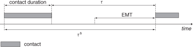
The two notions of inter-meeting time and contact duration are related as follows—see Figure 18.1:
![]()
From this formula, we can see that the two notions of inter-meeting time become nearly equivalent when the contact duration is much shorter than the time elapsing between consecutive meetings; that is, τs ≈ τ whenever δ ![]() τ.
τ.
Before concluding this chapter, it is worth observing that the mobility metrics defined above are based on a continuous-time model. They can be easily extended to a discrete-time model in those situations where the observation of the mobility and contact process occurs at periodic intervals, as is the case with real-world traces that have been studied in the opportunistic networking literature—see the next chapter.
Cai H and Eun D 2009 Crossing over the bounded domain: From exponential to power-law intermeeting time in mobil ad hoc networks. ACM/IEEE Transactions on Networking 17, 1578–1591.
Daly E and Haar M 2007 Social network analysis for routing in disconnected delay-tolerant MANETs. Proceedings of ACM MobiHoc, pp. 32–40.
Groenevelt R, Nain P and Koole G 2005 The message delay in mobile ad hoc networks. Performance Evaluation 62, 210–228.
Grossglauser M and Tse D 2002 Mobility increases the capacity of ad hoc wireless networks. ACM/IEEE Transactions on Networking 10(4), 477–486.
Hui P, Crowcroft J and Yoneki E 2008 BUBBLE Rap: Social-based forwarding in delay tolerant networks. Proceedings of ACM MobiHoc, pp. 241–250.
Karagiannis T, Le Boudec JY and Vojnovic M 2007 Power law and exponential decay of inter contact times between mobile devices. Proceedings of ACM Mobicom, pp. 183–194.
Spyropoulos T, Psounis K and Raghavendra C 2006 Performance analysis of mobility-assisted routing. Proceedings of ACM MobiHoc, pp. 49–60.
Spyropoulos T, Psounis K and Raghavendra C 2008a Efficient routing in intermittently connected mobile networks: The multi-copy case. ACM/IEEE Transactions on Networking 16, 77–90.
Spyropoulos T, Psounis K and Raghavendra C 2008b Efficient routing in intermittently connected mobile networks: The single-copy case. ACM/IEEE Transactions on Networking 16, 63–76.
Vahdat A and Becker D 2000 Epidemic routing for partially connected ad hoc networks. Technical Report CS-200006, Duke University.