
Chapter 19
Mobile Social Network Analysis
In the previous chapters, we introduced opportunistic networks and described the store, carry, and forward mechanism at the basis of message routing in this kind of network. Furthermore, we introduced the main metrics that have been defined to characterize mobility in opportunistic networks. In this chapter, we will focus attention on a specific type of opportunistic network, called the pocket-switched network (see also Chapter 17), in which the nodes forming the network are individuals carrying portable communication devices such as smart phones. This class of networks is very interesting from a mobility modeling perspective, since network nodes are carried by people, hence characterization of node mobility in PSNs is equivalent to characterization of human mobility, which is a very interesting topic investigated in many fields such as sociology, transportation engineering, urban planning, and so on. What is particularly interesting is trying to understand the relationships between social interactions among individuals, and their mobility pattern. Understanding these relationships is fundamental to, for example, optimize the performance of social-aware routing protocols, design social-aware communication primitives, design and optimize innovative services for mobile social networking applications, and so on.
In this chapter, we will present the state of the art on the characterization of human mobility patterns, based on an analysis of data traces obtained from real-world experiments. We will start by presenting the notion of a social network graph, which is useful for studying and characterizing social interactions among a set of individuals. We will then introduce the most relevant metrics used to characterize the structure of social network graphs, which can be used to identify the most “important” nodes in a social network graph, or to identify communities within a larger social structure. Finally, we will present the main findings of recent studies aimed at characterizing human mobility based on data trace analysis.
19.1 The Social Network Graph
A social network is a social structure made up of individuals and a set of connections between individuals representing some type of social interdependency, such as friendship, kinship, common interests, and so on. Social networks, which have been originally defined in field of sociology to, for example, measure social capital (i.e., the value that an individual gets from being part of a social structure), have now become a tool for explaining complex phenomena in different scientific fields such as anthropology, biology, economics, computer science, geography, and so on. For instance, social network analysis has been used in epidemiology to help understand how different human mobility patterns aid or inhibit the spread of infectious diseases such as HIV in a population. As another example, social networks are used to estimate the role of influential “opinion leaders” in spreading innovation within a population.
In a famous experiment performed in 1967, psychologist Stanley Milgram asked a sample of individuals in the USA to reach a particular target person by passing a message along a chain of acquaintances. Milgram then evaluated the average length of these message-passing chains, and established that five intermediaries—hence, six degrees of separation—were on average sufficient to connect an arbitrary pair of individuals. The fact that the chain of social acquaintances required to connect two arbitrary individuals in the world is in general short, and does not depend on the size of the population, is known as the small-world phenomenon, and was first noticed because of Milgram's experiment. Later on, small-world phenomena have been observed in many different types of social networks, such as the network formed by actors starring in the same movie, networks modeling hyperlinks in the World Wide Web, and so on.
The social network graph is a graph-based representation of a social network, where nodes correspond to social entities (e.g., individuals), and edges represent social ties between social entities. Depending on the specific social network considered, edges in the social network graph can be directed or undirected. In some cases, edges can be weighted, with the value of the weight representing the “intensity” of the social tie. In the following, we present some examples of social network graphs.
Based on Milgram's experiment, one can build a graph representing the social network underlying the experiment as follows: a node is assigned to each individual participating in the experiment, as the origin, target, or forwarder of a message; a directed edge is inserted between nodes u and v if node u passed a message to node v. The social network graph representing the Web is formed by adding a node for each url in the Web, and a direct edge between nodes u and v if page u contains a hyperlink to page v. A social network graph more relevant to PSNs of interest in this chapter is one in which nodes are the individuals forming the PSN, and there exists an edge between u and v if node u had at least a contact opportunity with node v during the period of interest. Alternatively, a weighted edge can be inserted, with a weight representing the number (or duration) of contact opportunities between the two nodes during the period of interest.
As the above examples highlight, in many cases social networks are very large, and are represented by graphs composed of several thousands (if not millions) of nodes and edges. For instance, the social network graph representing friendship relationships in an online social network application such as Facebook can be composed of up to several hundred million nodes and billions of edges. This explains why the field of social network analysis is closely related to the field of complex network analysis, an emerging research field at the intersection of many scientific disciplines such as mathematics, theoretical physics, computer science, biology, sociology, epidemiology, and so on. Complex networks are networks—represented as graphs—formed by a very large number of elements, and characterized by a non-trivial topology, which is neither regular nor entirely random.
The goal of social and complex network analysis is to provide a characterization of fundamental properties of the social (or complex) structure under study. For instance, typical goals of social/complex network analysis are the identification of “socially central” nodes (leaders) and the identification of “communities” within a larger network. To this end, several metrics have been defined on the social network graph, the most relevant of which are presented in the following section.
19.2 Centrality and Clustering Metrics
Several metrics have been defined on social network graphs to help understand and discover their structural properties. In the following, we introduce those metrics more relevant to the type of network under consideration in this part of the book, namely, PSNs. We first introduce a class of metrics aimed at measuring the “social centrality” of network nodes, and then a class of metrics aimed at measuring the degree of clustering observed in a network.
Before proceeding further, we observe that the metrics defined below can be applied to either the entire social network graph or a portion of it. Of particular importance is the so-called ego social network, that is, the portion of the social network as seen from a particular node in the network (the ego node). In graph-theoretic terms, the ego network of node u is the sub-graph of the social network graph formed by node u itself, by all the edges incident to u, and by all nodes which are endpoints of an edge incident to u. Ego networks are used sometimes as proxies of the complete social network graph, since it has been observed that, at least in some cases, the structural properties of ego networks are similar to those of the complete network (Marsden 2002).
19.2.1 Centrality Metrics
Centrality metrics are aimed at measuring the importance of a node within a large graph. When applied to social networks, centrality metrics are used to identify socially influential nodes. In the following, we introduce some relevant centrality metrics, and discuss how they have been used to optimize the performance of social-aware routing protocols for PSNs. Furthermore, we use G = (V, E) to denote a social network graph with node set V and (undirected) edge set E, and we assume G is connected.
A very simple centrality metric is node degree, that is, the number of edges in E incident to a node. Intuitively, nodes with higher degree have relatively more social ties, hence are socially better connected than nodes with relatively lower degree. However, it has been observed that, often, node degree is not sufficient to capture the “social importance” of a node within the network. For instance, a node which is part of a relatively isolated and tightly knit community within a larger network might have a relatively high degree because it has many connections with other members of its community, but nevertheless display a limited “social influence” due to the isolation of the community it belongs to. Justified by this observation, other metrics have been defined to measure node centrality.
A widely used centrality metric is betweenness centrality, which measures the fraction of shortest paths between any two nodes in the network that pass through a specific node. Formally, we have
![]()
where δst is the number of shortest paths from node s to node t in G, and δst(u) is the number of these paths passing through node u. The above value can be normalized by dividing it by (n − 1)(n − 2)/2, which represents the total number of node pairs in G which do not include u (n is the cardinality of the node set V). Betweenness centrality can be used, for instance, to measure how important a node is in spreading information within the social network: if a node u with high betweenness is removed from the network, the information will take much longer to spread throughout the network, since many shortest paths will no longer be available after node u's removal.
Another centrality metric is based on the topological notion of closeness, which, intuitively speaking, measures how “close” a node is to the other nodes in the network. Within the context of social networks, distance is defined in terms of number of hops in the social network graph, and it is called geodesic distance. Formally, the geodesic distance dG(u, v) between any two nodes in G is defined as the hop length of the shortest path connecting u and v in G. Closeness centrality is defined as follows:
![]()
Closeness centrality can be used, for instance, to measure how long it will take for a piece of information (message) generated at node u to reach all the other nodes in the social network.
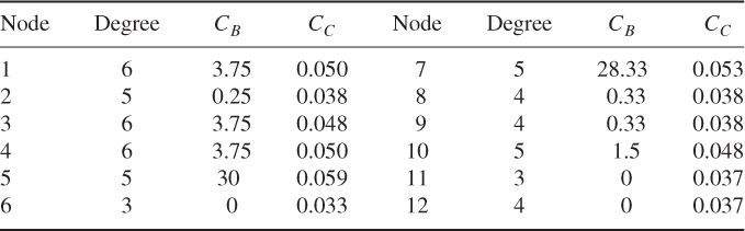
An example of a social network—based on Marsden (2002)—is shown in Figure 19.1, and the corresponding centrality metrics for each node are given in Table 19.1. The more central node(s) according to the different metrics are highlighted in Figure 19.1.
Figure 19.1 The bank wiring room social network (Marsden 2002). Nodes with the highest degree, betweenness centrality, and closeness centrality are highlighted in light gray (degree centrality) and dark gray (betweenness and closeness centrality).
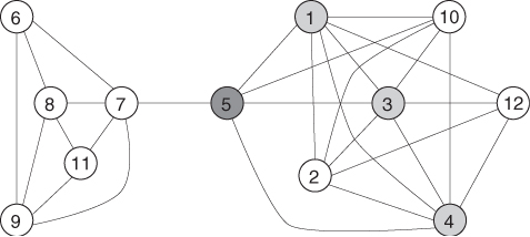
Table 19.1 Centrality metrics of the social network displayed in Figure 19.1
Centrality metrics have been used in the design of social-aware forwarding protocols for PSNs. The underlying idea is that relatively more central nodes in the social network graph should be preferred for carrying a copy of a message to relatively less central ones, since they have a higher likelihood of getting in touch with many other nodes within the PSN. Examples of protocols exploiting this idea are SimBet (Daly and Haar 2007) and BubbleRAP (Hui et al. 2008), which both use betweenness centrality (combined with other measures) to identify central nodes within the network.
19.2.2 Clustering Metrics
Clustering metrics are aimed at measuring the degree to which nodes in a graph tend to cluster together. In turn, clusters of nodes can be identified as communities within a larger social network.
In the following, we report the metric defined in Watts and Strogatz (1998), which is aimed at measuring the clustering as observed at a single node—that is, the clustering of a node's ego network. The clustering coefficient of node u quantifies how close its neighbors in G are to forming a clique (i.e., a complete graph). Formally, the clustering coefficient of node u is defined as follows:
![]()
where Eu is the set of edges in E such that both endpoints are neighbors of node u in G. In this formula, deg(u)(deg(u) − 1)/2 represents the total number of possible edges between any two neighbors of node u, where deg(u) is the degree of node u. Thus, the clustering coefficient represents the fraction of existing links between neighbors of u over the total number of possible such links. A clustering coefficient of 1 indicates that u's neighbors form a clique (maximal clustering), while a clustering coefficient of 0 indicates that u's neighbors are arranged as a star centered at u (minimal clustering).
Watts and Strogatz (1998) also define the network average clustering coefficient as the average of the clustering coefficients of all nodes in the network graph. The authors show that the network average clustering coefficient can be used to identify networks enjoying the small-world property: a network graph G = (V, E) is considered to have the small-world property if it has an average clustering coefficient significantly higher than that of a random graph with the same edge density constructed on V, and if the network graph has approximately the same average shortest path length as compared to the corresponding random graph.
While clustering metrics are aimed at measuring the level of clustering in a social network, they cannot be directly used to identify clusters (communities) within the network. Finding communities in a social network is a very important and challenging task that has been (and currently is) the subject of intensive research. Challenges in addressing this problem are related to the definition of community itself, which is not uniquely defined, and to the computational complexity of community detection algorithms, which are NP-hard in most cases.
Intuitively speaking, a community is a group of social entities within a larger social network displaying a large number of social ties between themselves. However, how to turn this intuitive notion into a formal, graph-theoretic definition is not straightforward. As a matter of fact, there is no universally accepted formal definition of community in the social and complex network literature.
We start by observing that community detection is a relevant problem only in sparse social networks, that is, in social networks where the average node degree is O(1), as is actually the case in most real-world social networks. If the number of edges in the social network graph is too large, then the distribution of edges among the nodes is likely to become too homogeneous for communities to exist.
To take a step forward toward a formal definition of community in a social network, we observe that, if we define as internal edges between community members, and as external edges joining a member of the community with a node outside the community, a community should satisfy the property that the number of internal edges is much larger than the number of external edges. Consider for instance the social network of Figure 19.1, where two communities can be clearly identified: a first community ![]() formed by nodes
formed by nodes ![]() = {6,7,8,9,11}, and a second community
= {6,7,8,9,11}, and a second community ![]() formed by nodes
formed by nodes ![]() = {1,2,3,4,5,10,12}. For community
= {1,2,3,4,5,10,12}. For community ![]() , the number of internal edges is 9, while the number of external edges is 1; for community
, the number of internal edges is 9, while the number of external edges is 1; for community ![]() , the number of internal edges is 16, while the number of external edges is 1. Thus, comparing the ratio of the number of internal edges to the number of external edges appears to be a good method for defining communities in a social network graph. Indeed, the above numbers should be normalized with respect to the maximum possible number of internal and external edges for a community
, the number of internal edges is 16, while the number of external edges is 1. Thus, comparing the ratio of the number of internal edges to the number of external edges appears to be a good method for defining communities in a social network graph. Indeed, the above numbers should be normalized with respect to the maximum possible number of internal and external edges for a community ![]() , which is
, which is ![]() and
and ![]() , respectively. However, this is a heuristic criterion to identify communities, and there is no consensus in the literature on the minimum value of the ratio that a community should satisfy, nor on whether computing the above ratio is the only method that can be used to determine whether a subset
, respectively. However, this is a heuristic criterion to identify communities, and there is no consensus in the literature on the minimum value of the ratio that a community should satisfy, nor on whether computing the above ratio is the only method that can be used to determine whether a subset ![]() of the network nodes V forms a community. Given this lack of consensus on a definition of community, the set of community detection algorithms proposed in the literature is even more heterogeneous.
of the network nodes V forms a community. Given this lack of consensus on a definition of community, the set of community detection algorithms proposed in the literature is even more heterogeneous.
While surveying the many definitions of community introduced in the literature and the related detection algorithms is far beyond the scope of this chapter (see Section 19.4 for reading suggestions on this topic), in the following we mention a very simple definition of community that is often used in the opportunistic networking literature.
A set of nodes ![]() can be defined as a community if the set of internal edges in
can be defined as a community if the set of internal edges in ![]() forms a clique. More formally, set
forms a clique. More formally, set ![]() is a community if and only if the number of internal edges is
is a community if and only if the number of internal edges is ![]() . Note that this definition accounts only for the number of internal edges to define a community, while the ratio between the number of internal and external edges is not considered. Thus, any subset of nodes V′ ⊆ V in a complete graph G = (V, E) would be regarded as a community according to this definition.
. Note that this definition accounts only for the number of internal edges to define a community, while the ratio between the number of internal and external edges is not considered. Thus, any subset of nodes V′ ⊆ V in a complete graph G = (V, E) would be regarded as a community according to this definition.
The above definition is very strict in defining a community, since each member of the community is required to have a social tie with every other member. Furthermore, under this definition all members in a community have symmetric connections, that is, there is no role differentiation within the community. This is in contrast to evidence from real-world observations clearly hinting at the existence of a whole hierarchy of roles within social communities. Despite these limitations, the above is the simplest possible definition of community, and it is often used in the opportunistic networking literature.
19.3 Characterizations of Human Mobility
A great deal of attention has been recently devoted to the characterization of human mobility patterns based on real-world data traces. In fact, several wireless network data traces became available in the literature (mostly through the CRAWDAD website (Team 2011)) starting in the early 2000s, and researchers have deeply studied these traces to gain an understanding of human mobility patterns not only qualitatively, but also quantitatively.
Roughly speaking, two types of data traces have been used to this end: location-based and contact-based traces. In the former, the location of the user is traced either directly (e.g., by recording the GPS reading), or indirectly (e.g., by recording the user's association with a WiFi access point or with a cellular base station). In the latter type of trace, logs of pairwise contacts–established, typically, through a short-range wireless technology such as WiFi or Bluetooth–between network users are recorded, while the location of users is typically not recorded in the data trace.
Wireless network data traces can be used to study features of individual human mobility patterns (e.g., how frequently individuals visit certain locations), as well as their contact patterns. Observe that only location-based traces can be used to study individual mobility patterns, while both location-based and contact-based traces can be used to characterize contact patterns between individuals. In case location-based traces are used for this purpose, pre-processing of the data trace is needed, in order to derive contact logs starting from user locations. Typically, it is assumed that two users are in contact if they are associated with the same access point/base station, or if they are within a certain distance from each other. Observe, though, that the pre-processing phase introduces an approximation in defining contact between users. Hence, contact-based traces should be preferred if the goal is to study contact patterns between users.
19.3.1 Characterization of Individual Human Mobility Patterns
We first present recent findings concerning the characterization of individual human mobility patterns, which are mostly due to a series of contributions from A.-L. Barabasi and colleagues (Gonzales et al. 2008; Song et al. 2010; Wang et al. 2011). The authors in their analyses consider large data sets of mobile phone users, whose trajectories and phone calls are traced for a relatively long time period (up to one year). More specifically, each time a user initiates or receives a call or SMS (Short Message Service), the cellular base station with which the user is currently associated is recorded in the trace. This type of trace allows, on the one hand, tracking the location of users with a spatial granularity corresponding to the average radio coverage area of a cellular base station–around a few square kilometers. On the other hand, these traces also allow tracking phone calls between users, so potentially giving information not only on their mobility patterns, but also on their social interactions (more specifically, those occurring through the cellular network).
The data traces used by these authors contain massive amounts of data (about 6 million users are traced for several months); however, there is a major drawback concerning the characterization of human mobility patterns: that is, the location of a user is tracked with uneven temporal resolution, since user location tracking occurs only when the user initiates or receives a call/SMS. Thus, it might very well be the case that the location of a user remains untracked for a relatively long period of time (up to several hours), introducing inaccuracies in the location tracking process.
One of the data traces considered in Song et al. (2010), though, does not have this shortcoming, because it contains the location records of 1000 users who signed up for a location-based service; hence, their location is tracked with a one-hour granularity, independently of whether they initiate/receive phone calls/SMSs. What is reported in the following is mostly based on the analysis of this data trace.
The following metrics have been considered to characterize individual human mobility:
Concerning displacement, it is observed that Δr follows a truncated power law with a cutoff at about 100 km, roughly corresponding to the maximum distance an individual can cover in one hour. More specifically, we have
![]()
where Δr is expressed in kilometers and α ≈ 0.55.
A similar law governs the waiting time, which also obeys a truncated power law with a cutoff at about 17 hours, approximately corresponding to a user's daily awake period. More specifically, we have
![]()
where β ≈ 0.8.
The number of locations visited within time t follows a power law with exponent 0.6, that is,
![]()
Finally, the visitation frequency closely resembles Zipf's law,
![]()
where fk represents the visitation frequency of the kth most visited location.
An interesting question to investigate is whether well-known mobility models such as random walks and Lévy flights are consistent with the above findings obtained from data traces, and whether they can be used to accurately model human mobility. Recall that Lévy flights in particular have been shown in the literature to faithfully reproduce animal movements. The analysis reported in Song et al. (2010) shows that random walks and Lévy flights cannot be used to faithfully reproduce human mobility patterns. In fact, if human mobility were to follow a random walk, we would have that the exponent of the law describing the number of locations visited with increasing time should be approximately equal to parameter β in the waiting time distribution. Based on the data traces, though, we have that this exponent is 0.6 ≠ β = 0.8. Similarly, if human mobility were to obey the Lévy flight model, the exponent of the law governing S(t) should be 1, instead of 0.6 as observed from the data traces. Similar conclusions can be drawn for the visitation frequency, which would be constant under either random walk or Lévy flight mobility, while it is instead distributed according to Zipf's law based on data trace analysis.
From the previous observations, it can be concluded that, unlike animal mobility, human mobility cannot be accurately modeled by random walk-like models. This is essentially due to fundamental differences in how random walk-like models and human mobility deal with the following factors:
As we will see in the next chapter, the above observations have motivated researchers to define mobility models specifically aimed at faithfully reproducing individual human mobility patterns.
Before ending this subsection, we want to mention the study reported by Wang et al. (2011), who show that mobility patterns and social networks are correlated. In other words, if two users display similar mobility patterns in visiting similar locations at similar times, they are likely to be “close” to each other in the social network graph, where the social network graph in Wang et al. (2011) is built based on phone calls between users. Mobility models aimed at modeling the interplay between human mobility and social relationships will also be discussed in the next chapter.
19.3.2 Characterization of Pairwise Contact Patterns
While the results presented above are useful for gaining an understanding of human mobility in general, what is important in opportunistic network performance evaluation is characterizing the pairwise contact pattern between individuals, namely, the duration and frequency of contact opportunities between an arbitrary pair of nodes in the opportunistic network. The studies on individual human mobility patterns can only partially be exploited for this purpose; in fact, their focus is mostly on the mobility pattern of each individual, and information about pairwise mobility metrics (e.g., how often two individuals are registered with the same base station) is often disregarded. Furthermore, the spatial granularity of the traces based on cellular networks is in the order of a few square kilometers, so it is too coarse to accurately estimate whether two individuals are within each other's WiFi/Bluetooth communication range even if they are registered with the same cellular base station.
To gain a deeper understanding of the statistical properties of contact patterns between pairs of individuals, a series of experiments have been performed in the past, where short-range radio devices (mostly based on Bluetooth technology) have been given to a number of volunteers. The devices were programmed to periodically activate the radio interface and perform an inquiry to discover other devices within communication range. The typical inquiry period is in the order of a few minutes, and it is thus much shorter than that used in the location-based data trace analyzed in Song et al. (2010). Thus, not only is the spatial resolution of the data traces used to characterize contact patterns smaller than that used in the characterization of individual human mobility patterns, but also the temporal resolution is much smaller (a few minutes instead of hours). Note that using a smaller spatial and temporal resolution is a prerequisite for accurate characterization of contact patterns. In fact, given that the communication range in opportunistic networks is short (in the order of a few tens of meters at most), movements of even a few tens of meters–which are small movements at the spatial granularity considered in cellular networks–are very important to determine whether a contact opportunity arises. In turn, since even small movements can determine whether a contact opportunity arises or not, the temporal granularity used to produce the data trace should also be small enough to capture such small movements.
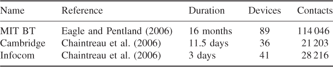
In this section, we report results on the characterization of pairwise contact opportunities mostly taken from Karagiannis et al. (2007), who conducted the first thorough study on this topic. The results are based on the analysis of six data traces, three of which were produced using Bluetooth devices. The features of these data traces are given in Table 19.2. The time granularity of the data traces is 300 s for the MIT BT trace, and 120 s for the Cambridge and Infocom data traces.
Table 19.2 Main features of the data traces analyzed in Karagiannis et al. (2007)
Karagiannis et al. (2007) were interested in characterizing the inter-meeting time distribution, where the inter-meeting time between nodes A and B is defined, we recall, as the time elapsing between the end of a contact between A and B and the beginning of the next contact between A and B.
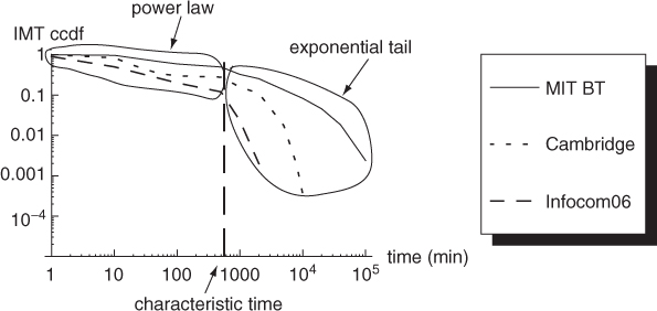
The main finding of Karagiannis et al. (2007) is that the inter-meeting time distribution displays a dichotomy: initially, it behaves like a power law, but the tail of the distribution is exponentially distributed. In other words, the inter-meeting time distribution behaves like a truncated power law. This can be seen from Figure 19.2 showing, for each data trace, the complementary cumulative density function of the inter-meeting time in log–log scale. The plots are initially linear, which, in log–log scale, corresponds to a power law, but, after a certain time, they display a sharp fall with time. Interestingly, the time at which the transition between power-law and exponential trend occurs (called the characteristic time) is approximately the same for the three data traces, being approximately equal to 12 hours. This fact clearly hints at a periodicity of human contact patterns similar to that displayed by individual movement patterns.
Figure 19.2 Complementary cumulative density function of the inter-meeting time distribution of the three data traces given in Table 19.2.
To investigate possible reasons for the displayed power-law and exponential tail dichotomy of the inter-meeting time distribution, Karagiannis et al. (2007) analyze the return time of a user to her/his home location, which is defined as the location where the user spends most of the time during the period of observation. To characterize return time, the authors use a set of location-based data traces containing GPS and cell phone tracks. The analysis reveals that the distribution of the return time to the home location displays the same dichotomy observed in the inter-meeting time distribution, with an initial power-law trend followed by an exponential drop-off. Driven by this observation, Karagiannis et al. (2007) formulate and validate the following hypothesis:
Inter-meeting time hypothesis: any two users in the opportunistic network tend to repeatedly meet at the same location, called the “meeting location.”
The inter-meeting time hypothesis is validated on the data traces, verifying that for about 80% of all the possible user pairs in the trace, more than 90% of the meetings occurs in at most two locations.
Summarizing, we can empirically explain the observed power-law and exponential tail dichotomy of the inter-meeting time as follows: the initial power-law trend is dictated by occasional meeting opportunities in the “outside world”; as time goes by, the inter-meeting time complementary cumulative density function displays a sharp drop-off, which is explained by the fact that nodes, if not meeting earlier in the “outside world,” tend to periodically meet at their “meeting location.”
As we will see in the next chapter, the inter-meeting time hypothesis is at the basis of recently proposed mobility models for opportunistic networks aimed at capturing the unique features of individual human mobility and contact patterns described in this chapter.
19.4 Further Reading
The reader interested in gaining a better understanding of the field of social and complex network analysis is referred to the following books: Easley and Kleinberg 2010; Newman (2010), and Newman et al. 2006. See also recent surveys on selected topics, such as the exhaustive survey by Fortunato (2006) on community detection.
Chaintreau A, Hui P, Crowcroft J, Diot C, Gass R and Scott J 2006 Impact of human mobility on the design of opportunistic forwarding algorithms. Proceedings of IEEE Infocom, pp. 1–13.
Daly E and Haar M 2007 Social network analysis for routing in disconnected delay-tolerant MANETs. Proceedings of ACM MobiHoc, pp. 32–40.
Eagle N and Pentland A 2006 Reality mining: Sensing complex social systems. Journal of Personal and Ubiquitous Computing 10, 255–268.
Easley D and Kleinberg J 2010 Networks, Crowds, and Markets: Reasoning about a Highly Connected World. Cambridge University Press, New York, US.
Gonzales M, Hidalgo C and Barabasi AL 2008 Understanding individual human mobility patterns. Nature 453, 779–782.
Hui P, Crowcroft J and Yoneki E 2008 BUBBLE Rap: Social-based forwarding in delay tolerant networks. Proceedings of ACM MobiHoc, pp. 241–250.
Karagiannis T, Le Boudec JY and Vojnovic M 2007 Power law and exponential decay of inter contact times between mobile devices. Proceedings of ACM Mobicom, pp. 183–194.
Marsden P 2002 Egocentric and sociocentric measures of network centrality. Social Networks 24, 407–422.
Newman M, Barabasi AL and Watts DJ 2006 The Structure and Dynamics of Networks. Princeton University Press, New Jersey, US.
Song T, Wang P and Barabasi AL 2010 Modelling the scaling properties of human mobility. Nature Physics 7, 713–718.
Team C 2011 http://crawdad.cs.dartmouth.edu/index.php.
Wang D, Pedreschi D, Song C, Giannotti F and Barabasi AL 2011 Human mobility, social ties, and link prediction. Proceedings of the ACM Conference on Knowledge Discovery and Data Mining (KDD), pp. 1100–1108.
Watts D and Strogatz S 1998 Collective dynamics of small-world networks. Nature 393, 440–442.