Chapter 20

Social-Based Mobility Models

As seen in the previous chapter, human mobility—and the resulting pairwise contact patterns—is characterized by features that make it substantially different from mobility patterns generated by simple mobility models such as random walks. In particular, human mobility has been recently shown to be influenced by, and to influence, social interactions between individuals. Given the above observations, researchers have recently proposed mobility models specifically designed to take the interplay between human mobility and social interactions into account.

In this chapter, we will present a set of recently proposed social-based mobility models aimed at faithfully reproducing individual human mobility patterns, and the resulting pairwise contact patterns. We will start by presenting a weighted version of the popular random waypoint model aimed at modeling different degrees of popularity in waypoint selection, and a mobility model where node movement is biased toward sub-areas (communities) specific to each node. We will then introduce a community-based mobility model, where an input social network graph is used to shape the mobility pattern of nodes in a network. The fourth model considered builds upon the notion of “home location” resulting from recent studies on human mobility characterization, and proposes a tradeoff between distance from home and popularity of the destination to determine individual mobility patterns. Another model, inspired by the principle of least action walking, is aimed at reproducing a set of features observed in human mobility traces concerning length of trips, pause time duration, inter-contact time, etc. Finally, we will present a contact-based mobility model which, instead of modeling the location of network nodes in a metric space, and then inferring contact patterns based on distance between nodes, is aimed at synthetically generating pairwise contact patterns directly. By exploiting the notion of “home location,” this contact-based mobility model is shown to be able to faithfully reproduce contact patterns observed in real-world data traces.

Before we present the social-based mobility models, the reader might wonder about the actual need for defining synthetic human mobility models, given the availability of a relatively large collection of wireless network traces in the literature. Although a number of mobility traces are actually available in the literature, and despite the extensive use of these traces in the opportunistic networking literature, synthetic mobility models still provide benefits to the network designer by allowing the variation of many network parameters (number of nodes, density of nodes, average number of contacts, and so on), which is only partially possible with real-world data traces. Thus, a quite common methodology in opportunistic network performance evaluation is to run the protocol under test on a few real-world data traces, as well as on synthetically generated traces typically obtained for larger network sizes than those of the networks used to produce the real-world traces.

20.1 The Weighted Random Waypoint Mobility Model

The weighted random waypoint mobility model was introduced in Hsu et al. (2005) with the aim of more faithfully reproducing human mobility. In particular, the authors focus on pedestrian mobility in a typical university campus.

The ideas underlying the weighted random waypoint mobility model are as follows:

To faithfully calibrate the mobility model for location popularity, pause time distributions, etc., Hsu et al. (2005) conduct a mobility survey targeted at a random set of 268 students on the campus. In the survey, students are requested to supply the following information: current location (building), previous visited location, next location to be visited, and pause time at each of these three locations.

The data collected from the survey is then processed to obtain popularity and pause time distributions as follows. First, the campus buildings are grouped into four categories: classrooms, libraries, cafeterias, and others. Further, a fifth category is introduced to model off-campus mobility. The pause time distributions for each location category are directly obtained from the survey data. The movement area is then divided into different regions as shown in Figure 20.1, which are modeled based on the University of Southern California campus where the survey was conducted. Movement between locations is driven by popularity, as determined by the mobility survey. In particular, a Markov chain (see Figure 20.1) is used to model transition probabilities between the five location categories. It is important to observe that, in accordance with what was observed in the survey data, the transition matrix of the Markov chain is time dependent. In particular, two transition matrices are defined: one for modeling movements in the morning (from 9 AM to 1 PM), and one for modeling movements in the afternoon (from 1 AM to 5 PM).

Figure 20.1 The weighted waypoint mobility model. The movement region is divided into five location categories (left): classrooms (CL), cafeterias (Ca), libraries (L), others on campus locations, and off campus. Movement between locations is governed by a five-state Markov chain (right), with transition probabilities derived from survey data.

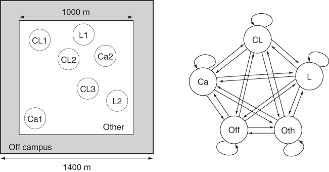
Summarizing, in the weighted random waypoint mobility model a node is given an initial location based on popularity (computed as the stationary distribution of finding a node at a certain location in the underlying Markov chain); then, the node remains in the selected location for a pause time drawn from the location-dependent pause time distribution; when the pause time elapses, a new location is selected based on the Markov chain transition matrix, and so on.

20.2 The Time-Variant Community Mobility Model

The weighted waypoint mobility model presented in the previous section introduces some realistic aspects into the waypoint mobility model, such as the fact that different waypoints display different degrees of popularity, that waypoint popularity changes with time, and that pause time distribution is waypoint dependent. However, similar to the original RWP model, each mobile node in the weighted waypoint mobility model behaves identically (from a stochastic perspective). This is an unrealistic aspect of the mobility model described in the previous section, since in the real world different individuals display stochastically different mobility patterns.

The time-variant community (TVC) mobility model was introduced in Hsu et al. (2007) to account for heterogeneous individual mobility patterns. The model is designed also to account for other features observed in human mobility patterns, such as skewed location popularity distribution, time-variant mobility patterns, and periodical reappearance of nodes at the same location.

In order to create skewed location visiting preferences, each node in the network is randomly assigned to a subregion of the mobility region R, called its community—similar to the notion of “home location” used in other mobility models. A node tends to visit its community relatively more often than regions residing outside the community. The notion of community is also useful to model heterogeneous node mobility patterns: since communities are chosen randomly, and in general are different for different nodes, the resulting mobility patterns clearly have different stochastic properties.

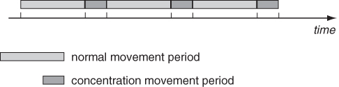
In order to reproduce periodical reappearance of a node at the same location, time in the TVC model is divided into two alternate phases, called normal movement periods and concentration movement periods—see Figure 20.2. During concentration movement periods, the likelihood of performing movements within a node's community is even higher than in normal movement periods, implying that the node is likely to visit its community periodically.

Figure 20.2 The TVC mobility model alternates between normal and concentration movement periods.

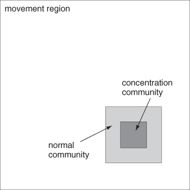
In TVC, communities are defined as square subregions of the movement region R, with a different side during the normal and concentration movement periods—see Figure 20.3. Notice that, depending on the scenario, the concentration community can be smaller than (as in Figure 20.3), larger than, or have the same size as the normal community.

Figure 20.3 Normal and concentration communities in the TVC mobility model.

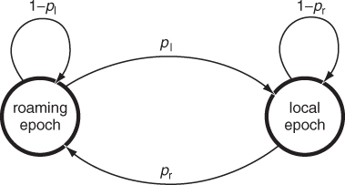
During each time period, a node has two different movement modes, called local epoch and roaming epoch. During a local epoch, node movement is confined within the current community. In a roaming epoch, the node is free to move in the entire movement region R. The rule used to select speed is the same as in the RWP model: before initiating a new trip, a node chooses a speed uniformly at random in an interval [v_min, v_max], and the speed is kept constant for the entire trip. The length of a trip is drawn from an exponential distribution with average trip length equal to a parameter , while trip direction is chosen uniformly at random in the [0, 2π] interval (random direction mobility). The toroidal wrap-around rule is used in case a node hits the boundary of the allowed movement region (the community in local epochs, or the entire movement region R in roaming epochs). When the trip ends, the node pauses at the current location for a time drawn uniformly at random in a [0, T_max] interval before starting a new trip.

Alternation between local and roaming epochs during a movement period is governed by the two-state Markov chain depicted in Figure 20.4, with probabilities p_l and p_r determining transition into local and roaming epoch state, respectively. Notice that these transition probabilities can be different in the normal and concentration movement periods.

Figure 20.4 Two-state Markov chain governing transitions between local and roaming epochs in the TVC mobility model.

Hsu et al. (2007) derive formulas for approximating two important mobility metrics of the TVC mobility model, namely, the expected hitting time and the expected meeting time—see Chapter 18 for a formal definition of these metrics. The expressions approximating the expected hitting and meeting times with TVC mobility are cumbersome, and for this reason we do not report them here. The interested reader is referred to Hsu et al. (2007).

Besides providing explicit formulas for approximating the expected hitting and meeting times, Hsu et al. (2007) also provide a validation of the TVC mobility model based on a comparison to real-world traces, showing that the TVC mobility model achieves the design goals of reproducing skewed location visiting preferences and periodical reappearance of a node at the same location.

20.3 The Community-Based Mobility Model

Musolesi and Mascolo (2007) define a mobility model which explicitly takes into account social relationships between users to define mobility patterns. The model is based on the observation that human mobility is influenced by the social relationships between individuals. Thus, the authors suggest starting the definition of the mobility model from an input social network graph, which describes the social relationships between the individuals forming the network.

The block diagram of the community-based mobility model is shown in Figure 20.5. Mobility modeling is a five-step process:

1. Social graph definition: the first step consists of defining a social network graph modeling social relationships between individuals. In principle, any (undirected) social network graph can be used for this purpose. The graph can be obtained from real-world data; alternatively, the authors endow the model with an algorithm for producing synthetic, yet realistic, social network graphs (see further on in this section).

2. Community detection: after the social network graph is produced, a community detection algorithm is run to identify (non-overlapping) communities in the graph. In general, any community detection algorithm can be used for this purpose. In the implementation of their model, Musolesi and Mascolo (2007) use the algorithm proposed in Newman and Girvan (2004), which repeatedly removes edges incident to nodes with maximal betweenness centrality to partition the social network graph into disjoint communities.

3. “Home location” generator: the next step consists of assigning a “home location” to each community in the social network graph. To this end, the movement area is divided into a number of square cells (assumed to be much larger than the number of communities in the social network graph), and a community is assigned a square cell chosen uniformly at random as its “home location,” with the constraint that no two communities can be assigned to the same cell.

4. Initial node position generator: then, initial node positions are generated as follows: a node belonging to community is positioned uniformly at random in the square cell corresponding to the “home location” of community .

5. Movement generation: after the four steps above have been performed, actual movement of nodes can start. Node movement obeys a weighted waypoint mobility rule, where the weight of waypoints is determined by the strength of social ties (see below for details).

Figure 20.5 Block diagram of the community-based mobility model.

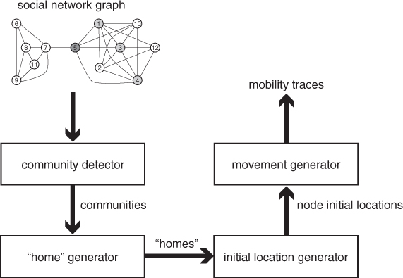
The social network graph defined in step 1 is assumed to be a weighted, undirected graph G = (V, E), where the weight of edge (u, v) represents the intensity of the (symmetric) social relationship between node u and node  v. Before computing the community structure, graph G is turned into an unweighted graph G_σ by defining a threshold σ: in G_σ, only edges in G with weight ≥ σ are retained.

As mentioned above, besides allowing use of an arbitrary social network graph G as input, the community-based mobility model provides the user with an algorithm for producing synthetic, yet realistic, social network graphs. The algorithm used to generate synthetic social network graphs is based on the caveman model introduced in Watts (1999): initially, K fully connected graphs (corresponding to communities, called caves in this model) are added to the social network graph; then, every edge of this initial graph is rewired to point to another cave with a certain, fixed probability p. This simple algorithm has been shown by Watts (1999) to produce realistic social network graphs, characterized by a relatively high average clustering coefficient and a relatively low average path length.

Node movement after initial deployment obeys the following rules. Each node is assigned a goal, roughly corresponding to the popular notion of waypoint. More formally, node u is said to be associated with a certain cell C_{i, j} (i and j are the cell indexes) if its current goal is located within C_{i, j}. Note that the fact that node u is associated with cell C_{i, j} does not necessarily imply that it is currently located in C_{i, j}, but instead means that its current movement destination is within C_{i, j}.

Goals are assigned to nodes according to the following rule. Assume node u has reached its previous goal, and needs to select a new goal at time t; let N_{i, j}(t) be the number of nodes associated with cell C_{i, j} at time t. The following metric is used to define the social attractivity a certain cell exerts on node u:

where w_uv is the weight of the edge connecting u and v in G—set to 0 if there is no edge between u and v in G.

The movement generator allows for two possible alternative mechanisms to select the next goal:

After the next goal is selected, the node starts moving toward the goal along a straight-line trajectory, with a fixed speed chosen uniformly at random in a certain interval—this part of the model is identical to RWP mobility.

An interesting feature of the community-based mobility model is that it allows the social network graph to be periodically changed, so as to induce different mobility patterns at different times of the day—which is a typical feature of human mobility, as discussed in the previous chapter. When the input social network graph changes, so does the community structure, and the mapping of nodes to home locations; hence, node mobility patterns will gradually tend to change to reflect the different structure of the underlying social network graph.

To validate the model, Musolesi and Mascolo (2007) compares sample synthetic traces produced by the community-based model to the Cambridge data trace (Chaintreau et al. 2006). The metrics considered in the comparison are the inter-meeting time and the contact duration. For the sake of comparison, the authors consider also the well-known RWP model. Synthetic and RWP traces are obtained by placing 100 nodes in a square movement region of side 5 km, and choosing movement speeds uniformly at random in the [1, 6] m/s interval. For the sake of “home location” computation in the community-based model, the movement region is divided into 625 squares of side 200 m. Contact patterns between nodes are generated under the assumption that nodes have a transmission range of 250 m.

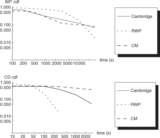
The cumulative distribution of inter-meeting and contact duration obtained from simulations is shown in Figure 20.6. As can be seen from the figure, by suitably tuning parameter p used in the generation of the social network graph with the caveman model, the community-based mobility model can be made to produce contact patterns quite similar to those encountered in the Cambridge data trace, especially for the inter-meeting time. This is evidently not the case for the RWP mobility model, which produces contact patterns very different from those displayed by the data trace.

Figure 20.6 Inter-meeting time (top) and contact duration (bottom) distributions of the Cambridge data trace, RWP mobility model, and community-based mobility model. Rewiring probability p in the community-based mobility model is set to 0.2.

20.4 The SWIM Mobility Model

Mei and Stefa (2009) introduced the SWIM (Small World In Motion) mobility model, which is designed to be a simple mobility model able to faithfully reproduce contact patterns between individuals. The intuition behind SWIM is as follows: people tend to visit more often places not too far from their home, and where they can meet lots of other people. In other words, Mei and Stefa (2009) identify two major factors influencing individual human mobility: proximity to home and popularity of the destination. In particular, the authors assume a tradeoff between these two factors when designing SWIM, observing that an individual typically travels a long distance only to reach a very popular location.

Other important observations on which SWIM is based are the following:

The SWIM mobility model operates in a number of steps, described below:

1. Initialization: before starting the simulation, the movement region is divided into a number of square cells, which are used to assign “homes” and destinations to mobile nodes. In particular, the authors assume the side of a cell to be small enough to enable direct communication between any two nodes located in the same cell. In other words, if the node's transmission range is set to r, the side of square cells is set to . After square cell partitioning, each node u is assigned a “home” cell C(u) uniformly at random, and its initial position is chosen uniformly at random in cell C(u).

2. Destination selection: for each node u, the next destination (waypoint) is chosen uniformly at random in the destination cell, which is selected uniformly at random according to a weighted probability distribution. More specifically, for each cell C_{i, j} in the movement region, the following metric relative to node u is computed and used to probabilistically select the destination cell:

where dist(pos(u), C_{i, j}) is a function that decays as a power law with the distance between the position pos(u) of node u and the center of cell C_{i, j}, seen(C_{i, j}) is the number of nodes seen at C_{i, j} the last time node u visited C_{i, j}—initialized to 0 for all the C_{i, j} at the beginning of the simulation—and α is a constant in the [0, 1] interval.

3. Waiting time selection: the waiting time at the current location is chosen according to a power law with slope 1.45 and upper bound of 4 hours.

4. Movement phase: as the waiting time elapses, the node starts moving toward the next destination along a straight-line trajectory, with a speed proportional to the distance to be traveled. More specifically, to simplify the model definition as much as possible the authors assume that if the distance to be covered is d, the node speed is d/k meters per second, implying that each trip in SWIM has the same duration of k seconds.

As can be seen from the above description, SWIM is designed to be very simple, with only a few parameters available to tune its mobility characteristics. In particular, parameter α has a major effect on mobility patterns, allowing the “home proximity” vs. “popularity” tradeoff to be tuned: the larger the value of α, the more the nodes tend to repeatedly visit locations close to home; on the contrary, smaller values of α give rise to mobility patterns with nodes tending to visit quite distant, yet popular, locations.

Note that, unlike the community-based mobility model described in the previous section, social interactions between individuals are indirectly accounted for in SWIM: in particular, a node's mobility pattern is influenced by other nodes' mobility patterns through function seen(), which records the number of nodes encountered in a cell during the most recent visit.

Mei and Stefa (2009) evaluate SWIM ability to faithfully reproduce human contact patterns both theoretically and through simulation. In particular, the authors formally prove that the tail of the inter-meeting time distribution generated by SWIM is exponentially distributed, and use simulations to assess that the head of the distribution is a power law, thus showing that the traces generated by SWIM display the power-law and exponential tail dichotomy of the inter-meeting time distribution observed by Karagiannis et al. (2007).

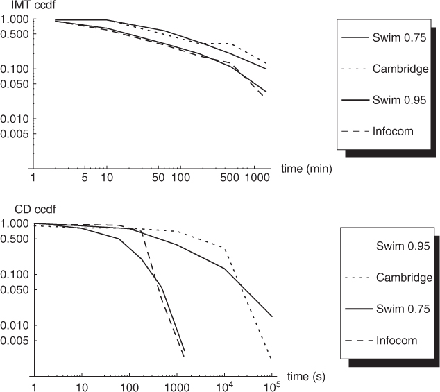
Mei and Stefa (2009) compare the contact patterns generated by SWIM to those of three data traces, including the Cambridge and Infocom traces given in Table 19.2. In Figure 20.7, we show the complementary cumulative density function of the inter-meeting time and contact duration distributions obtained with SWIM and with the Cambridge and Infocom traces. The SWIM traces have been produced as follows. In order to closely match the conditions under which the real-world data traces were produced, a square movement region of side 300 m is considered, and nodes are assumed to have a transmission range of 30 m. Function dist() is set as follows:

where c_{i, j} is the point corresponding to the center of cell C_{i, j}. Parameter α is optimized to reproduce contact patterns of real-world traces as faithfully as possible, and it is set to 0.75 in the SWIM trace resembling the Infocom trace and to 0.95 in the other trace. As seen in the plots displayed in Figure 19.7, by properly tuning parameter α the SWIM model is able to reproduce real-world contact patterns quite accurately.

Figure 20.7 Inter-meeting time (top) and contact duration (bottom) distributions of the Cambridge and Infocom data traces, and SWIM mobility model with parameter α set to 0.95 and 0.75, respectively.

In a recent paper Mei et al. (2011) propose a variation of the SWIM model aimed at explicitly taking into account the similarity of user interests when associating “home” location to nodes. More specifically, each node in the network is associated with an interest profile, which is an m-dimensional vector in the [0, 1]^m interest space modeling a node's interest along m possible dimensions. An interest dimension in Mei et al. (2011) is intended as modeling interest in a certain topic (e.g., music, books, cinema, etc.), as well as individual habits (e.g., living in a certain neighborhood, working in a certain place, etc.). A similarity metric is defined on the interest space to express similarity between individual interests, thus expressing “homophily” between individuals. In social science, the notion of “homophily” expresses the fact that two individuals share similar interests.

The goal of the modified SWIM model defined in Mei et al. (2011) is to produce contact traces where nodes with relatively more similar interests are relatively more likely to meet than nodes with diverse interests. This is motivated by sociological studies showing that there exists a positive correlation between “homophily” between individuals and the frequency/duration of their contacts (McPherson 2001). Positive correlation between similarity of individual interests and contact frequency/duration has been observed also by Mei et al. (2011) and Noulas et al. (2009) based on the Infocom data trace, for which not only logs of pairwise contacts are available, but also anonymized profiles of the individuals who participated in the experiment.

In Mei et al. (2011), it is proposed to change the “home” location assignment in SWIM as follows. Instead of assigning the “home” location to nodes uniformly at random in the movement region, allocation is performed based on the similarity of user interests, with the goal of assigning nodes with relatively similar interests to relatively close “home” locations. This way, given the SWIM mobility pattern according to which nodes return to their home quite frequently, nodes with relatively similar interests tend to meet relatively more often than nodes with diverse interests. These authors propose to allocate nodes to “home” locations as follows. First, two out of the m possible interest dimensions are chosen. The specific values of node u along these directions give the location of node u's home, after suitable normalization of the movement region.

20.5 The Self-Similar Least Action Walk Model

The mobility models described so far have the common property of selecting a new destination at a time, subject to some random rule. In real life, however, human movements are often planned: given a set of locations to visit in a forthcoming period of time (e.g., workplace, the shopping mall, a fitness center, a school, etc.), an individual plans an itinerary to visit all locations, with the goal, typically, of reducing distance traveled or trip time. The ability of an individual to plan an itinerary across a set of locations to visit is not captured by models where trips are selected one after the other, as in the models described so far in this chapter.

The self-similar least action walk (SLAW) model was introduced in Lee et al. (2009) with the aim of modeling the above-described trip planning ability of humans. The model is inspired by the least action principle, according to which all objects (humans in this context) move in the direction of minimizing their discomfort (traveled distance in this context). The intuition is that, when planning an itinerary, people tend to reduce the distance traveled by visiting all nearby locations before visiting farther destinations, unless some high-priority events such as appointments induce them to overrule the above strategy.

The SLAW model which we describe in this section is shown by Lee et al. (2009) to fulfill several properties typical of human mobility patterns, as derived from analysis of real-world mobility traces (recall Chapter 19):

It is interesting to observe that the above properties are closely interrelated: Lee et al. (2009) show that fractal destinations (4) induce truncated power-law trip length (1). Hong et al. (2008) show that mobility patterns confined in a restricted area (2) give rise to the power-law and exponential time dichotomy of inter-contact times (3).

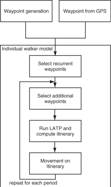
The block diagram of the SLAW mobility model is shown in Figure 20.8. Initially, a large population of possible destinations (waypoints) is generated. Waypoints are generated so as to satisfy the self-similarity principle (see Lee et al. (2008) for details). Alternatively, waypoints can be extracted from an existing GPS trace. These waypoints constitute the universe W of all possible destinations for all nodes in the network. In order to satisfy property 2 of heterogeneous node mobility patterns, an individual walker model is then implemented. In order to diversify individual mobility patterns, a subset W′ of waypoints is randomly extracted from W, corresponding to the recurrent destinations of a specific node. Note that different nodes in general have different recurrent destinations, although overlapping between sets W′ is possible. After selecting set W′, a set of waypoints is chosen to form an itinerary for the current period. The period is defined in SLAW to be approximately 12 hours. The destination set for the period is composed of the set W′ or recurrent waypoints, augmented with a set W′′ of additional waypoints chosen from W − W′ in order to increase randomness in movement patterns and mixing of individual trajectories. The set W′ ∪ W′′ of waypoints for the current period is then given as input to the least action trip planning (LATP) module, which randomly computes the itinerary for the current period satisfying the least action principle (on average). Once the itinerary is computed, the set of movements for the current period is performed; each time a node reaches a destination, it pauses for a random time drawn from a truncated power law.

Figure 20.8 Block diagram of the SLAW mobility model.

It is important to observe that particular care should be taken in selecting the individual set of recurrent waypoints in step 1 of the individual walker model. In fact, recurrent waypoints should be selected so as to satisfy the self-similarity principle, which is not necessarily guaranteed by the fact that the set W of all possible destinations from which set W′ is chosen does satisfy self-similarity. To preserve self-similarity also on subset W′, the following random selection procedure is implemented. First, waypoints in W are clustered by connecting together waypoints that are less than 100 m apart. Denoting by the set of clusters and by |X| the cardinality of set X, we have that each cluster C_i in is assigned weight w_i = |C_i|/|W|. Each individual walker then selects k clusters from with probability proportional to the weights w_i, where k = 3 − 5 is a parameter of the model. Then, for each selected cluster C_i, 5 to 10% (the exact percentage of selected waypoints is another parameter of the model) of the waypoints in C_i are chosen uniformly at random and added to the set W′ of recurrent destinations.

The additional waypoints in step 2 of the individual walker model are selected as follows. A cluster C_j is selected uniformly at random from the clusters in not used to extract waypoints in W′. Then, 5 to 10% of the waypoints in C_j are selected uniformly at random and constitute set W′′ for the current period.

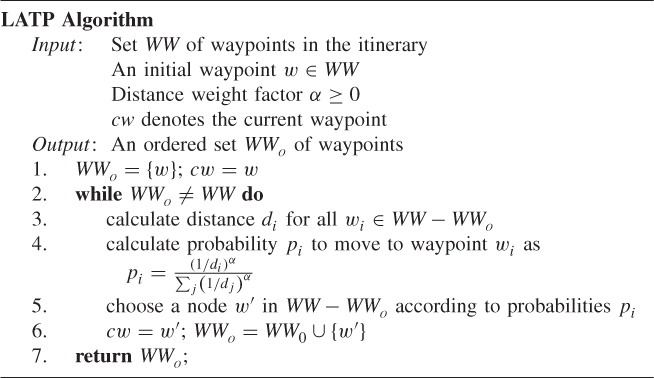
The LATP module of SLAW is shown in Figure 20.9. Given an unordered set WW of waypoints to visit and an initial waypoint w, the algorithm returns an ordered set WW_o of all waypoints in WW, starting from w. The ordered set is formed in an incremental way: given the current waypoint, the next point is randomly selected according to a distance-weighted probability distribution. Parameter α is used to tune obedience to the least action principle: for large values of α, selection of the next waypoint becomes a quasi-deterministic process based on distance to the current waypoint; on the other hand, if α = 0 the next waypoint is chosen uniformly at random.

Figure 20.9 The LATP algorithm in SLAW.

20.6 The Home-MEG Model

In the previous sections, we introduced representative mobility models taking into account the social dimension of human mobility. A common characteristic of these models is that they model human mobility in a metric space, and then derive pairwise contact patterns—which are used to validate the accuracy of the mobility model through comparison to real-world data traces—based on node trajectories combined with a notion of transmission range. Since the main goal of a mobility model for opportunistic networks is to generate realistic pairwise contact patterns between network nodes, some authors have proposed models aimed at directly modeling the occurrence/disappearance of pairwise wireless links between individuals, without modeling physical individual mobility in an underlying metric space. This approach has the potential advantage of producing simpler models of contact patterns amenable for use in protocol performance analysis, while not sacrificing accuracy in the generated contact patterns.

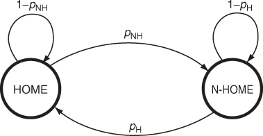
Becchetti et al. (2011) introduce the Home-MEG (Markovian Evolving Graph) model to model the occurrence/disappearance of wireless links between pairs of individuals. The Home-MEG model is a discrete-time model, according to which existence of the link between u and v can change state at time t, t + 1, … and so on. The model is based on the well-known observation made by Karagiannis et al. (2007) that pairs of individuals tend to repeatedly meet in a few locations, known as “home” (or “meeting”) location. Thus, taking an arbitrary pair u, v of individuals in the network, the wireless link between these nodes can be modeled according to the two-states transition diagram shown in Figure 20.10. The wireless link between u and v can be in one of two possible states: the “Home” state corresponds to the situation in which both nodes are in the “home” location, while the “Not-Home” state corresponds to the situation in which one of the two nodes (or both) is not in the “home” location. In accordance with Karagiannis et al. (2007), the instantaneous probability for link (u, v) to exist at any time t is p_h, with 0 < p_h < 1, when the link is in state “Home,” while it is p_l, with 0 ≤ p_l < p_h, when the link is in state “Not-Home.” Besides p_h and p_l, the Home-MEG model has two more parameters, p_H and p_NH, determining the transition probabilities between the two possible link states at each time instant.

Figure 20.10 Pairwise link state transition diagram in the Home-MEG model.

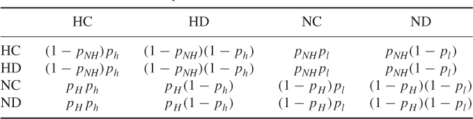
It is easy to see that the existence/non-existence of any pairwise link in the Home-MEG model can be modeled with a four-states Markov chain, where the states are HC and NC modeling the existence of the link (u, v) when the link is in state “Home” and “Not-Home,” respectively, and HD and ND modeling the non-existence of the link when in state “Home” and “Not-Home,” respectively. The corresponding transition matrix is given in Table 20.1.

Table 20.1 Transition matrix of the Markov chain used to model existence/non-existence of a pairwise wireless link in the Home-MEG model

In order to reproduce pairwise contact patterns in a network with n nodes, it is sufficient to generate n(n − 1)/2 identical and independent copies of the above Markov chain (one for each possible pairwise link) in the network.

It is important to observe that the notion of “Home” state in the Home-MEG model is referred to a specific node pair, and, in particular, the transitive property does not hold. In other words, the fact that the pairs of nodes u, v and u, w are in the “Home” state does not imply that pair v, w are also in the “Home” state. This is a consequence of the fact that the n(n − 1)/2 copies of the Markov chain modeling a single link in the network are independent. Thus, the “Home” state in the Home-MEG model must not be intended as a single popular location within the network where all the nodes regularly meet, but rather as a location where a specific pair of nodes regularly meet, where meeting locations are assumed to be different for each pair of nodes. Admittedly, this is an approximation of reality, where meeting locations are likely to be shared by several pairs of nodes. However, in the following we show that, despite this approximation, the Home-MEG model is able to accurately reproduce the aggregate inter-contact time distribution observed in several real-world traces.

Summarizing, the Home-MEG model has four parameters: parameters p_H and p_NH used to tune the transition between the “Home” and “Not-Home” states, and parameters p_h and p_l used to set the probability of link existence in the two states.

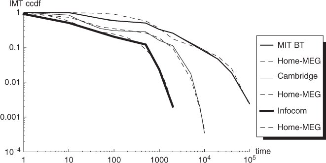
Becchetti et al. (2011) verify the accuracy of the contact traces generated by the Home-MEG model by comparing the synthetic traces produced by the Home-MEG model to the six data traces used in Karagiannis et al. (2007). In particular, Becchetti et al. (2011) consider the inter-meeting time distribution to assess the accuracy of the Home-MEG traces. The four parameters of the Home-MEG model are optimized to match the real-world data traces through an iterative search process over the four-dimensional parameter space. The inter-meeting time complementary cumulative density function of the Home-MEG traces vs. the three traces given in Table 19.2 is shown in Figure 20.11, and the corresponding optimal parameters for the Home-MEG model are given in Table 20.2. As can be seen from the plots, the Home-MEG model, if suitably tuned, is able to accurately reproduce pairwise contact patterns observed in real-world traces. It is also interesting to observe that, while optimal Home-MEG parameters for the three real-world traces are quite different in absolute terms, their relative values are quite similar, hinting at the following guidelines for Home-MEG model parameter tuning:

Table 20.2 Optimal parameters of the Home-MEG model for the three data traces shown in Figure 20.11

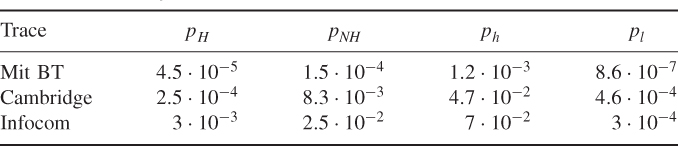
Figure 20.11 Inter-meeting time complementary cumulative density function of the MIT BT, Cambridge, and Infocom data traces, and of the synthetic traces produced with the Home-MEG model. The time step in the Home-MEG model is set to 82 s.

In Chapter 22, we will see how to exploit these guidelines in the analysis of asymptotic broadcast time in opportunistic networks through the Home-MEG model.

20.7 Further Reading

This chapter presented a non-exhaustive survey of mobility models aimed at modeling individual human mobility, including human “social” behavior. Other models have been proposed in the literature, such as the Truncated Levy Walk model (Rhee et al. 2008), the Working Day Movement model (Ekman et al. 2008), and the Home-cell Community-based Mobility Model (Boldrini and Passarella 2010). We refer the reader to the respective papers for details.

References

Becchetti L, Clementi A, Pasquale F, Resta G, Santi P and Silvestri R 2011 Information spreading in opportunistic networks is fast. Internet draft: available at http://arxiv.org/abs/1107.5241.

Boldrini C and Passarella A 2010 HCMM: Modeling spatial and temporal properties of human mobility driven by users' social relationships. Computer Communications 33, 1056–1074.

Chaintreau A, Hui P, Crowcroft J, Diot C, Gass R and Scott J 2006 Impact of human mobility on the design of opportunistic forwarding algorithms. Proceedings of IEEE Infocom, pp. 1–13.

Ekman F, Keranen A, Karvo J and Ott J 2008 Working day movement model. Proceedings of the ACM Workshop on Mobility Models, pp. 33–40.

Hong S, Rhee I, Kim S, Lee K and Chong S 2008 Routing performance analysis of human-driven delay tolerant networks using the truncated Levy walk model. Proceedings of the ACM Workshop on Mobility Models, pp. 25–32.

Hsu WJ, Merchant K, Shu HW, Hsu CH and Helmy A 2005 Weighted waypoint mobility model and its impact on ad hoc networks. Mobile Computing and Communications Review 9, 59–63.

Hsu WJ, Spyropoulos T, Psounis K and Helmy A 2007 Modeling time-variant user mobility in wireless mobile networks. Proceedings of IEEE Infocom, pp. 758–766.

Karagiannis T, Le Boudec JY and Vojnovic M 2007 Power law and exponential decay of inter contact times between mobile devices. Proceedings of ACM Mobicom, pp. 183–194.

Lee K, Hong S, Kim S, Rhee I and Chong S 2008 Demystifying the Levy walk patterns in human walks. Technical Report, North Carolina State University, pp. 1–14.

Lee K, Hong S, Kim S, Rhee I and Chong S 2009 SLAW: A new mobility model for human walks. Proceedings of IEEE Infocom, pp. 855–863.

McPherson M 2001 Birds of a feather: Homophily in social networks. Annual Review of Sociology 27(1), 415–444.

Mei A and Stefa J 2009 SWIM: A simple model to generate small mobile worlds. Proceedings of IEEE Infocom, pp. 2106–2113.

Mei A, Morabito G, Santi P and Stefa J 2011 Social-aware stateless forwarding in pocket switched networks. Proceedings of IEEE Infocom, pp. 251–255.

Musolesi M and Mascolo C 2007 Designing mobility models based on social network theory. Mobile Computing and Communications Review 11, 1–11.

Newman M and Girvan M 2004 Finding and evaluating community structure in networks. Physical Review E.

Noulas A, Musolesi M, Pontil M and Mascolo C 2009 Inferring interests from mobility and social interactions. Proceedings of the Workshop on Analyzing Networks and Learning with Graphs.

Rhee I, Shin M, Hong S, Lee K and Chong S 2008 On the Levy walk nature of human mobility. Proceedings of IEEE Infocom, pp. 924–932.

Watts D 1999 Small Worlds: The Dynamics of Networks between Order and Randomness. Princeton University Press, Princeton, NJ.