Appendix B
Elements of Graph Theory, Asymptotic Notation, and Miscellaneous Notions
In this appendix, we start by introducing the asymptotic notation, and then report basic definitions and concepts from graph theory that have been used in this book. We will also formally define miscellaneous notions used in the book, such as linearity of operators, convexity and concavity, and so on. Most of the material presented in this appendix are based on Bollobàs (1985) and Bollobàs (1988), on Appendix B of Santi (2005), and on online resources such as Wikipedia and Wolfram MathWorld.
B.1 Asymptotic Notation
Definition B.1 (Big-O notation)
Let
f(
n) and
g(
n) be two functions defined on

. One can write
f(
n) =
O(
g(
n)) if and only if there exist a positive real number
c and a real number
n0 such that

The big-O notation is used to express the fact that, as the argument n of the function grows larger, function f(n) is upper bounded by function g(n), up to a constant factor.
Definition B.2 (Big-Omega notation)
Let
f(
n) and
g(
n) be two functions defined on

. One can write
f(
n) = Ω(
g(
n)) if and only if there exist a positive real number
c and a real number
n0 such that

The big-Omega notation is used to express the fact that, as the argument n of the function grows larger, function f(n) is lower bounded by function g(n), up to a constant factor.
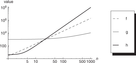
The intuition behind the big-O and big-Omega notation is pictorially represented in Figure B.1. The figure shows the behavior for increasing values of n of the three functions

For small values of n, function g(n) is larger than both f(n) and h(n), due to the large constants in the polynomial. However, as n grows larger, the dominating terms in the three functions become n2 for f(n), n for g(n), and n3 for h(n). This explains why, for large enough values of n (say, n > 30), we have h(n) > f(n) > g(n). Using asymptotic notation, we have
1. f(n) = Ω(g(n)) and f(n) = O(h(n));
2. g(n) = O(f(n)) and g(n) = O(h(n));
3. h(n) = Ω(f(n)) and h(n) = Ω(g(n)).
Definition B.3 (Big-Theta notation)
Let
f(
n) and
g(
n) be two functions defined on

. One can write
f(
n) = Θ(
g(
n)) if and only if there exist positive real numbers
c1,
c2 and real number
n0 such that

Alternatively, one can define that f(n) = Θ(g(n)) if and only if f(n) = O(g(n)) and f(n) = Ω(g(n)).
The big-Theta notation is used to express the fact that, as the argument n of the function grows larger, function f(n) is both upper and lower bounded by function g(n), up to a constant factor.
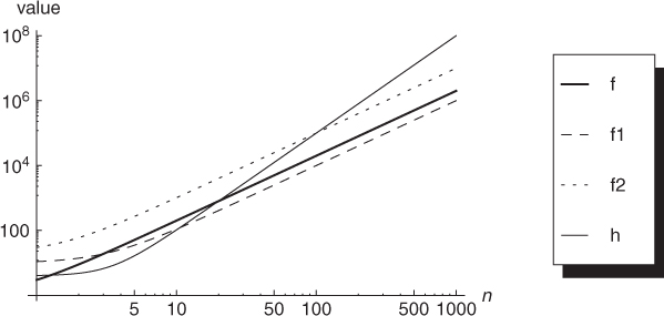
The intuition behind the notion of big-Theta notation is pictorially represented in Figure B.2. The figure shows the behavior for increasing values of n of function f(n) as defined above, and of the two functions

Although functions f, f1, and f2 differ in their constant terms, their asymptotic behavior is dominated by the n2 term, hence it is equivalent (up to a constant factor). This fact can clearly be seen from Figure B.2 which shows, for comparison, also the plot of a function with different asymptotic behavior (namely, function h(n) as defined above).
Definition B.4 (Tilde notation)
Let
f(
n) and
g(
n) be two functions defined on

. One can write
f(
n) = Õ(
g(
n)) if and only if there exists a positive real number
c such that
f(
n) =
O(
g(
n)log
cn). Notation

and

can be defined similarly.
Definition B.5 (Small-o notation)
Let
f(
n) and
g(
n) be two functions defined on

. One can write
f(
n) =
o(
g(
n)) if and only if for every positive real number ϵ there exists a real number
nϵ such that

If g(n) is non-zero (at least for sufficiently large n), we can equivalently define f(n) = o(g(n)) to hold if and only if
The small-o notation is used to express the fact that function f(n) is asymptotically dominated by function g(n).
Definition B.6 (Small-omega notation)
Let
f(
n) and
g(
n) be two functions defined on

. One can write
f(
n) = ω(
g(
n)) if and only if for every positive real number
k there exists a real number
nk such that

If g(n) is non-zero (at least for sufficiently large n), we can equivalently define f(n) = ω(g(n)) to hold if and only if
The small-omega notation is used to express the fact that function f(n) asymptotically dominates function g(n).
B.2 Elements of Graph Theory
Definition B.7 (Graph)
A graph G is an ordered pair of disjoint sets (V, E), where E ⊆ V × V. Set V is called the vertex, or node, set, while set E is the edge set of graph G. Typically, it is assumed that self-loops (i.e., edges of the form (u, u), for some u ∈ V) are not contained in a graph.
Definition B.8 (Order of a graph)
The order of graph G = (V, E) is the number of nodes in G, that is, the cardinality of set V.
Definition B.9 (Directed and undirected graph)
A graph G = (V, E) is directed if the edge set is composed of ordered node pairs. A graph is undirected if the edge set is composed of unordered node pairs.
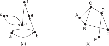
Examples of directed and undirected graphs are reported in Figure B.3 Unless otherwise stated, in the following by graph we mean undirected graph.
Definition B.10 (Weighted graph)
A weighted graph is a graph in which edges, or nodes, or both, are labeled with a weight.
Definition B.11 (Neighbor nodes)
Given a graph G = (V, E), two nodes u, v ∈ V are said to be neighbors, or adjacent nodes, if (u, v) ∈ E. If G is directed, we distinguish between incoming neighbors of u (those nodes v ∈ V such that (v, u) ∈ E) and outgoing neighbors of u (those nodes v ∈ V such that (u, v) ∈ E).
Definition B.12 (Node degree)
Given a graph G = (V, E), the degree of a node u ∈ V is the number of its neighbors in the graph. Formally,

If G is directed, we distinguish between in-degree (number of incoming neighbors) and out-degree (number of outgoing neighbors) of a node.
For instance, node A in the undirected graph in Figure B.3 has degree 2, and its neighbors are nodes B and C. Node b in the directed graph in Figure B.3 has in-degree 1 and out-degree 2; its incoming neighbor is node a, while its outgoing neighbors are nodes a and e.
Definition B.13 (Regular graph)
A graph G = (V, E) is regular if all its nodes have the same degree. If the graph is directed, it is required that all the nodes in the graph have the same in-degree and out-degree. A regular graph where all nodes have degree k is called a k-regular graph.
Definition B.14 (Complete graph)
The complete graph Kn = (V, E) of order n is such that |V| = n, and E = V × V, that is, (u, v) ∈ E for any two distinct nodes u, v ∈ V. Otherwise stated, the complete graph of order n is the unique (n − 1)-regular graph of order n.
Definition B.15 (Square grid)
A toroidal square grid of side m is a 4-regular graph G = (V, E) in which nodes are arranged in the Euclidean plane at integer coordinates (0, 0), (0, 1), …, (m, m). The node at coordinates (i, j) in the grid has an edge to the four nodes at coordinates (i + 1, j), (i − 1, j), (i, j + 1), and (i, j − 1), where all the operations are modulo m. In a simple square grid of side m, wrap-around edges are omitted.
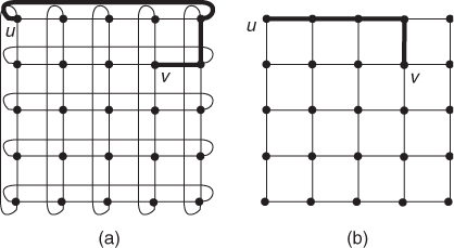
The toroidal and simple square grids of side 4 are shown in Figure B.4. Notice that the simple square grid is not a regular graph, since the corner nodes have degree 2, boundary nodes have degree 3, and internal nodes have degree 4.
Definition B.16 (Path)
Given a graph G = (V, E), and given any two nodes u, v ∈ V, a path connecting u and v in G is a sequence of nodes {u = u0, u1, …, uk−1, uk = v} such that for any i = 0, …, k − 1, (ui, ui+1) ∈ E. The length of the path is the number of edges in the path.
Definition B.17 ((Hop) distance)
Given a graph G = (V, E) and any two nodes u, v ∈ V, their distance dist(u, v) (also called hop distance, especially within the networking community) is the minimal length of a path connecting them. If there is no path connecting u and v in G, then dist(u, v) = ∞.
Definition B.18 (Manhattan distance)
Let
u = (
u1, …,
ud),
v = (
v1, …,
vd) be any two vectors in

, for some
d ≥ 1. The
Manhattan distance between
u and
v is defined as follows:
The notion of Manhattan distance can be equivalently defined on simple square grids G = (V, E) as follows: given any two nodes u, v ∈ V, the Manhattan distance between nodes u and v is the hop distance between the two nodes in the graph.
The Manhattan distance between nodes u, v in the simple square grid of Figure B.4 is 4; a minimum length path connecting u and v is shown in bold in the figure. Note that the notion of Manhattan distance is no longer equivalent to the notion of hop distance in toroidal square grids. In fact, the hop distance between nodes u and v in the toroidal square grid of Figure B.4 is 3 (see path in bold), while we have

Definition B.19 (Graph diameter)
The diameter of graph G = (V, E) is the maximum possible distance between any two nodes in G. Formally,
The distance between nodes a and e in the directed graph in Figure B.3 is 2, and the diameter of the graph is 5. The diameter of the undirected graph in Figure B.3 is 3.
Definition B.20 (Sub-graph)
Given a graph
G = (
V,
E), a
sub-graph of
G is any graph
G′ = (
V′,
E′) such that
V′ ⊆
V and
E′ ⊆
E. Given any subset
V′ of the nodes in
G, the sub-graph of
G induced by
V′ is defined as
, where
E(
V′) = {(
u,
v) ∈
E:
u,
v ∈
V′}, that is,

contains all the edges of
G such that both endpoints of the edge are in
V′.
Definition B.21 (Connected and strongly connected graph)
A graph G = (V, E) is connected if for any two nodes u, v ∈ E there exists a path from u to v in G. If G is directed, we say that G is strongly connected if for any two nodes u, v ∈ E there exist a path from u to v and a path from v to u in G.
The undirected graph in Figure B.3 is connected, while the directed graph in the same figure is not strongly connected. In fact, there exist a pair of nodes for which connecting paths in both directions do not exist. For instance, there is no path (neither direct, nor inverse) connecting node d with node f.
Definition B.22 (Tree)
A tree T = (V, E) is a connected graph with n nodes and n − 1 edges. That is, a tree is a minimally connected graph.
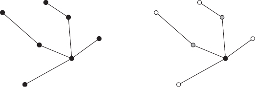
Definition B.23 (Rooted tree)
A rooted tree T = (V, E) is a tree in which one of the nodes is selected as the tree root. Once the root node r is chosen, the other nodes in the tree can be classified as either internal node or leaf node. An internal node u is such that there exists v ∈ V such that (u, v) ∈ E and dist(u, r) < dist(v, r). A leaf node l is such that, for any v ∈ V such that (l, v) ∈ E, then dist(l, r) > dist(v, r).
Figure B.5 displays examples of a tree and a rooted tree.
Definition B.24 (Random graph)
Two methods are commonly used to define random graphs. In the first method, due to Gilbert (1959), a
G(
n,
p)
random graph is built on
n nodes by including each of the
n(
n − 1)/2 possible edges in the graph independently with probability
p =
p(
n). In the second method, due to Erdos and Rény (1959) and

, a
G(
n,
M)
random graph of
n nodes is selected uniformly at random from the collection of all graphs with
n nodes and
M =
M(
n) edges.
Note that, due to the law of large numbers, the number of edges in a G(n, p) graph is approximately p · n(n − 1)/2, under the condition that p n2 → ∞. Then, under this condition, graph G(n, p) behaves similarly to graph G(n, p · n(n − 1)/2). Several asymptotic properties of random graphs such as connectivity, diameter, node degree, etc., have been studied in the literature. The interested reader is referred to Bollobás (1985).
B.3 Miscellaneous Notions
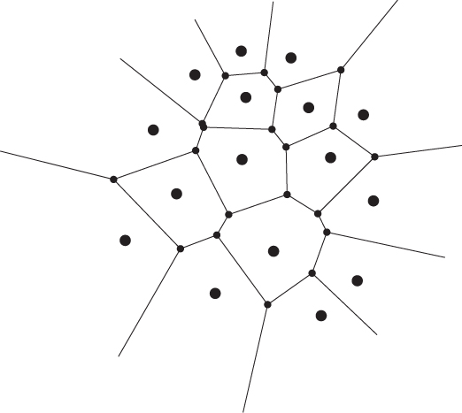
Definition B.25 (Voronoi diagram)
Let
be a set of points in a metric space
S. For definiteness, suppose
S is the Euclidean plane with the associated Euclidean distance. The
Voronoi diagram associated with set

is a tessellation of
S induced by a collection of
Voronoi cells 
, where Voronoi cells are defined as follows. The Voronoi cell
Ci associated with point

is the set of points in
S whose distance to
pi is not larger than the distance to any other point

. Formally,

where d() denotes distance in S.
An example of a Voronoi diagram computed starting from a set of 16 points in the Euclidean plane is shown in Figure B.6.
Definition B.26 (Convex function)
A function

defined on an interval
X is called
convex if, for any two points
x1,
x2 ∈
X and any
t ∈ [0, 1],

The function is said to be strictly convex if

for any t, with 0 < t < 1.
Definition B.27 (Concave function)
A function

defined on an interval
X is called
concave if function
g(
x) = −
f(
x) is convex in
X.
Strict concavity is defined similarly.
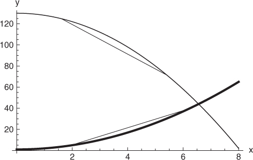
Informally speaking, a function is convex if the graph of the function lies below the line segment joining any two points in the graph. A concave function, instead, lies above the line segment joining any two points in the graph. See Figure B.7 for an example of convex and concave functions.
Definition B.28 (Convex set)
A set

is said to be
convex if, for any
x,
y ∈
C and any
t ∈ [0, 1], the point (1 −
t)
x +
ty is in
C. A set

that does not satisfy this condition is called a
non-convex set.
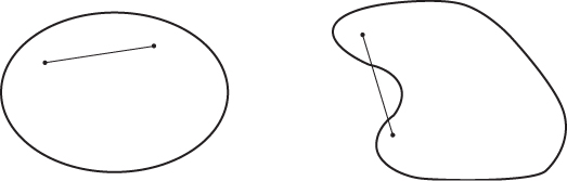
Informally speaking, a set C is convex if, for any two points x, y chosen in C, the line segment connecting points x and y is also within C. Examples of convex and non-convex sets are shown in Figure B.8. Notice that Voronoi cells are convex polygons—see Figure B.6. Notice also that the above definition of set convexity can be immediately extended to other vector spaces such as  for d > 2, etc.
Definition B.29 (Linear function)
A function

is
linear if, for any
, and any
,

The above definition of linearity can be easily extended to functions between two arbitrary vector spaces.
Definition B.30 (Pearson's correlation coefficient)
Let (X1, Y1), …, (Xn, Yn) be a collection of samples of random variables X and Y. The Pearson's correlation coefficient between X and Y is defined as follows:
where

and

denote the mean value of
X and
Y, respectively.
The Pearson's correlation coefficient takes values in [ − 1, 1], with − 1 and 1 representing maximum correlation between random variables X and Y (inverse and direct correlation, respectively), and 0 representing statistical independence.
References
Bollobás B 1985 Random Graphs. Academic Press, London.
Bollobás B 1998 Modern Graph Theory. Springer, New York.
Erdos P and Rény A 1959 On random graphs. Publicationes Mathematicae 6, 290–297.
Gilbert E 1959 Random graphs. Annals of Mathematical Statistics 30, 1141–1144.
Santi P 2005 Topology Control in Wireless Ad Hoc and Sensor Networks. John Wiley & Sons, Ltd, Chichester.