PICKING STOCKS

It is a difference of opinion that makes horse races.

—MARK TWAIN

The value-investing philosophy is simple: Look for great companies whose stocks are inexpensive relative to their dividends and earnings. It is pretty much the same philosophy held by John Burr Williams, Benjamin Graham, Warren Buffett, and other value investors—great companies at a fair price. Buffett has two advantages over us ordinary value investors. First, his reputation gives him sweetheart deals. Companies that want a public-relations stamp of approval sell stock to Buffett at bargain prices that aren’t available to the rest of us. Second, his insurance companies give him enormous leverage. When people buy insurance, their premiums plus whatever the company earns by investing the premiums are used to pay off claims for car insurance, home insurance, life insurance, and so on. Insurance companies set their premiums based on an assumption that they will earn modest returns—for example, Treasury rates—when they invest the premiums. Buffett’s insurance companies set premiums comparable to those set by other insurance companies, but then invest the premiums in stocks that, on average, do a lot better than Treasury bonds. In essence, Buffett borrows money from policyholders at Treasury rates (currently around 2 percent) and invests the premiums in stocks giving double-digit returns. You and I can’t borrow money at Treasury rates. But we can still be value investors.

The starting point is to identify great companies, then to decide whether their stocks are attractively priced. Let’s apply the JBW, Shiller, and Bogle valuation measures to the three top companies in Fortune’s 2016 list of most admired stocks: Apple, Google, and Amazon.

APPLE

When I was a graduate student during the years 1969–1971, Yale’s computer center was a brick building that had been home to an insurance company. There was a behemoth of a computer inside an air-conditioned and dust-controlled room. The rest of the building was row after row of keypunch machines that were used to prepare IBM punch cards. Students and professors sat at the keypunch machines, which were much like typewriters, and typed in data and software code, with each keystroke punching a hole in a card. Each card represented one line of instructions, so a complete program might fill several cardboard boxes, each holding 2,000 cards.

Computer users handed their boxes of cards to machine operators through a set of sliding glass windows, and the operators fed the cards into the giant computer. Users then waited for their output, which might take hours. If there were errors, users sifted through their cards looking for a mistake, corrected it, resubmitted their cards, and waited for the next round of output.

The never-ending click-clacking of the keypunch machines was awful, as were the long waits and treasure hunts for errors, but it was state of the art at the time. It was also stressful, and sometimes the stress got out of hand. One of my fellow PhD students, “Jack,” had worked for nearly a year trying to debug the program he needed to finish his thesis. One day, when he handed his two boxes of punch cards through the window to the machine operator, the operator turned to load the cards into the card feeder, but tripped and spilled thousands of cards on the floor. Jack jumped through window and tried to choke the operator. Two other people pulled Jack away and explained that it was a prank. They had distracted Jack and swapped his boxes for two boxes of surplus cards, which the operator proceeded to drop and scatter. Jack was relieved, but not amused.

When I came to Pomona College in 1981, the college was using dumb terminals (keyboards and display monitors) scattered around campus and connected to the college’s IBM mainframe. Dumb terminals were a big step up from punch cards, since the results came back quickly and the terminals were quiet!

However, the entire system was under the control of the computer center. The computer center decided what programs to put on the mainframe and they selected a relatively small number of programs that were easy for them to maintain. Users had few options.

Then came the personal computer revolution, so called because—unlike a dumb terminal—a personal computer has a built-in CPU and does not need to be connected to a mainframe. Users can choose the software they want, including software they have written themselves.

Pomona College’s computer center resisted the revolution because it was easier for them to maintain a small set of programs on a mainframe. As a user, it was clear to me that the personal computer revolution might be delayed, but it would not be stopped. My wife and I gave our first son an Apple II for his ninth birthday. When he opened the box, I took the instructions and he took the computer. He had it up and running before I finished reading the instructions.

Legendary mutual fund manager Peter Lynch said that some of his biggest winners came from going to a mall with his daughters, giving them some money, and seeing where they spent it. He argued, “If you like the store, chances are you’ll love the stock.” His shopping strategy might be justified by the argument that new stores fly under Wall Street’s radar. However, in lesser hands, his philosophy can lead investors to make the classic mistake of buying a stock because the company is great, not because the stock is cheap.

This was one of my (few) Peter Lynch moments. I knew that users wanted personal computers, not dumb terminals, and I saw firsthand how easy the Apple II was to use. Apple stock didn’t pay dividends and its earnings were dodgy, but I bought some stock anyway. I also bought my son Apple stock for his high school graduation present. In retrospect, I was lucky. Commodore, Kaypro, Tandy, and dozens of other PC makers did not survive. Apple was sometimes near-death.

Apple has evolved into a mature company that derives most of its revenue from its iPhones, which, like the Macintosh and Apple II, were revolutionary. Apple still makes computers, of course, and has a solid Apple-ecosystem that is used by millions of Apple fans. Apple is now a money machine that can be assessed by value investors.

Let’s value Apple today (August 2016) using the same three valuation methods we used to value the S&P 500 in Chapter 12: the JBW equation, Shiller’s cyclically adjusted price-earnings ratio (CAPE), and the Bogle model.

The John Burr Williams (JBW) equation is

where R is the total annual return, D is the annual dividend, P is the current stock price, and g is the annual rate of growth of dividends.

For Apple stock in August 2016, the annual dividend was $2.28 per share and the stock price was around $100, giving a dividend yield of 2.28 percent:

In my assessment of the S&P 500, I assumed a 5 percent growth rate of dividends, roughly the long-run growth rate of dividends and the U.S. economy. Using that 5 percent growth rate here implies a 7.28 percent total return, which (as Table 13-1 shows) is 5.47 percentage points above the ten-year Treasury rate.

At the time, Apple’s 2.28 percent dividend yield was slightly higher than that for the S&P 500, making it a slightly more attractive stock if we use the same 5 percent dividend growth rate for Apple and the S&P 500. This seems extremely conservative. Apple’s dividends had increased by 10 percent a year since Apple instituted a dividend in 2012 and Apple’s earnings per share had increased at a 55 percent annual rate over the past ten years and at a 41 percent annual rate over the previous five years.

Many feared that Apple was no longer a premier growth stock, that it was now just a mature money machine. It certainly gets harder to maintain a crazy growth rate as a company gets larger; but, even so, it was hard to imagine that Apple would grow more slowly than the average company in the S&P 500 over the next ten years. Plus, there is nothing inherently bad about being a mature money machine. In fact, it may be a safer investment than a young start-up with nothing more than hoped-for profits in the future.

Apple had been No. 1 in the annual Forbes ratings of the most admired companies for nine years running, 2008 through 2016. A sudden collapse seemed unlikely.

Apple’s earnings certainly wouldn’t grow by 40 or 50 percent forever, nor would its dividends grow by 10 percent forever, but a 5 percent growth rate for dividends was surely conservative.

I also made a more complicated calculation of the present value of Apple’s dividends, assuming that Apple’s dividends grow at 10 percent a year for twenty years, then drop to a 5 percent growth rate, roughly the projected long-run growth rate of the economy.

We can calculate the present value of these projected dividends for any assumed required return. This is the intrinsic value of Apple stock. It turns out that if we discount the projected dividends by a 9.54 percent required return, the intrinsic value is $100.

Here are the implications:

1.Investors who would be happy with a 9.54 percent annual rate of return should be happy owning Apple stock.

2.If dividends grow more than assumed in these calculations, the return is even larger.

3.If dividends grow less than anticipated, the return is smaller; for example, if Apple’s dividend growth rate drops to 5 percent after ten years, the return is 8.41 percent; if it falls to 5 percent immediately, the return is 7.28 percent.

This all makes sense. A 2.28 percent dividend yield gives a 7.28 percent return if dividends grow by 5 percent a year forever and a 12.28 percent return if dividends grow by 10 percent a year forever. If the dividend growth rate is 10 percent for a while and then drops to 5 percent, the return will be between 7.28 percent and 12.28 percent, and the return will be higher the longer the 10 percent growth rate is maintained.

Are these calculations dependent on the heroic assumption that Apple will be around forever? Not really. The heavy discounting of distant dividends makes them essentially meaningless.

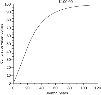
Figure 13-1 shows the cumulative intrinsic value of Apple’s dividends, using a 9.54 percent required return. For example, the cumulative value over a twenty-year horizon is the present value of the first twenty years of dividends. As shown, almost all of Apple’s intrinsic value comes from the first 100 years. If Apple were to disappear 100 years from now, it would have essentially no effect on Apple’s current intrinsic value.

(Nonetheless, it is good to use a model that assumes an infinite horizon, because it keeps us from guessing about what the price of Apple stock will be tomorrow or a year from now. The infinite-horizon model makes no assumptions about the future price of Apple stock.)

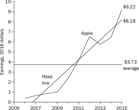
Now let’s try Shiller’s model. The cyclically adjusted P/E ratio (CAPE) can be misleading for individual companies that have been growing very rapidly. Figure 13-2 shows that Apple’s earnings per share (in 2016 dollars) increased from $0.38 per share in 2006 to $9.22 per share in 2015, a 43 percent annual rate of increase. Because of Apple’s rapid growth, the $3.73 average over this ten-year period greatly understates Apple’s current and projected future earnings.

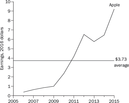
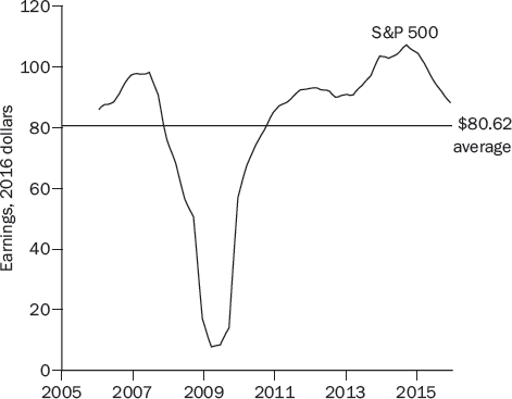
Figure 13-3 shows the S&P 500’s inflation-adjusted earnings. Here, the fluctuations around the average are more important than the growth in earnings over time, and it makes sense to calculate a ten-year average in order to smooth out these fluctuations and give a more accurate representation of earnings than would be provided by any single year. For Apple, in contrast, the growth over time is more important than the year-to-year fluctuations, and the ten-year average is a misleading representation of Apple’s earnings.

Nonetheless, I calculated the cyclically adjusted earnings yield (CAEP) by dividing Apple’s average inflation-adjusted earnings by the inflation-adjusted price of Apple stock ($100):

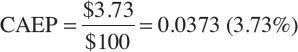
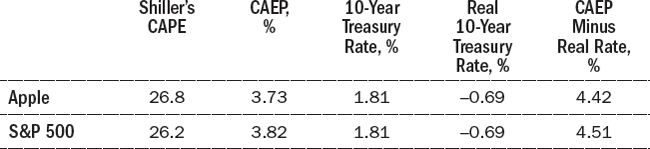
Since the earnings yield is a rough estimate of the real rate of return on stocks, I compared CAEP to the real interest rate on ten-year Treasury bonds.

Table 13-2 shows the calculations, using an assumed 2.5 percent rate of inflation, the average over the past several years. Apple was slightly less attractive than the overall S&P 500, but there was still a 4.42 percentage-point difference between the Apple’s cyclically adjusted earnings yield and the real return on ten-year Treasury bonds. Taking into account the conservative $3.73 number for Apple’s earnings, Apple becomes more attractive.

This, too, makes sense. With Apple stock at $100 a share, a cyclically adjusted earnings figure of $3.73 gives an earnings yield of 3.73 percent, which is an estimate of the real return on Apple stock.

Cyclically adjusted earnings are intended to adjust for the ups and downs in business cycles. Movements in Apple’s earnings during the years 2006 through 2015 were not due to a business cycle, but to Apple’s growth. Its 2015 earnings of $9.22 don’t really need be adjusted much for the business cycle, so it is reasonable to use an earnings figure that is closer to $9.22 than $3.73, which gives a projected real return substantially higher than the already attractive 3.73 percent.

One way to adjust a growth company’s earnings for the business cycle is to fit a line to the earnings data, as in Figure 13-4. The fitted line smooths out the year-to-year fluctuations, as intended, but allows for growth. By this reckoning, Apple’s 2015 cyclically adjusted earnings were $8.18, giving a CAEP of 8.18 percent, more than double the value using the ten-year average earnings of $3.73:

This projected real return of 8.18 percent is 8.87 percent higher than the projected real return on ten-year Treasury bonds.

Let’s now look at John Bogle’s model for estimating stock returns over a ten-year horizon:

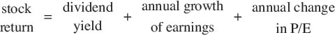
Apple’s price-earnings ratio was 12 in August 2016, half that of the S&P 500. Table 13-3 shows the returns predicted by the Bogle model for the assumption that the price-earnings ratios in 2026 are still 12 for Apple and 24 for the S&P 500, and that both earnings grow at 5 percent annually. If the price-earnings ratio is constant and earnings are projected to grow at the same rate as dividends, Bogle’s model and the JBW equation give the same total return values. Table 13-3 also shows the total returns if Apple’s earnings grow at 10 percent annually for the next ten years, and if Apple and the S&P 500 both have a P/E of 20 in 2026. Since Apple’s P/E would be going up and the S&P 500 P/E would be going down, this enhances Apple’s return and diminishes the S&P 500 return.

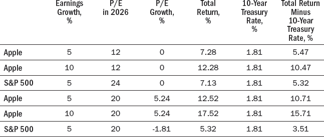
As with the JBW and Shiller metrics, the Bogle model’s implications make sense. In 2016, Apple had a dividend yield of 2.28 percent. If its dividends and earnings were to grow at 5 percent a year for ten years, and its P/E stays at 12, it will give investors a 7.28 percent return over this ten-year horizon. If Apple’s earnings and dividends grow by more than 5 percent a year over the next ten years and/or its P/E is higher than 12 in 2026, the rate of return on Apple stock will be higher than 7.28 percent—perhaps much higher.

Table 13-4 summarizes the calculations for these three models. I concluded that the S&P 500 was an attractive investment and that Apple was even more so. In August 2016, I held an imprudently large fraction of my portfolio in Apple stock.

	Total Return Minus Treasury Rate, %
DIVIDEND-DISCOUNT MODELS
Apple, JBW with 5% dividend growth	5.47
Apple, dividend discount with 10% growth for 10 years, 5% afterward	6.60
Apple, dividend discount with 10% growth for 20 years, 5% afterward	7.73
S&P 500, JBW with 5% dividend growth	5.32
SHILLER MODEL
Apple, with CAEP = 3.73%	4.42
Apple, with CAEP = 8.18%	8.87
S&P 500, with CAEP = 3.82%	4.51
BOGLE MODEL
Apple, with 5% earnings growth and P/E = 12 in 2026	5.47
Apple, with 10% earnings growth and P/E = 12 in 2026	10.47
S&P 500, with 5% earnings growth and P/E = 24 in 2026	5.32
Apple, with 5% earnings growth and P/E = 20 in 2026	10.71
Apple, with 10% earnings growth and P/E = 20 in 2026	15.71
S&P 500, with 5% earnings growth and P/E = 20 in 2026	3.51

GOOGLE

In January 1994, just as the World Wide Web (WWW) was starting to get traction, two Stanford graduate students, Jerry Yang and David Filo, started a website. “Jerry and David’s Guide to the World Wide Web” was a list of what they considered interesting web pages. A year later, they incorporated the company with the sexy name Yahoo. By now, they had a catalog of 10,000 sites and 100,000 Yahoo users a day, fueled by the fact that the popular Netscape browser had a Directory button that sent people to Yahoo.com.

As the Web took off, Yahoo hired hundreds of people to search for sites to add to its exponentially growing directory. They added graphics, news stories, and advertisements. By 1996, Yahoo had more than 10 million visitors a day. Yahoo thought of itself as a media company, sort of like Fortune magazine, where people came to be informed and entertained and advertisers paid for a chance to catch readers’ wandering eyes. Yahoo hired its own writers to create unique content. As Yahoo added more content, such as sports and finance pages, it attracted targeted advertising—directed at people who are interested in sports or finance. Yahoo started Yahoo Mail, Yahoo Shopping, and other bolt-ons.

Then came Google in 1998 with its revolutionary search algorithm. Yahoo couldn’t manually keep up with the growth of the Web, so it used Google’s search engine for four years while it developed a competing algorithm. Meanwhile, Google established itself as the go-to search site and maintained a 90 percent worldwide share of the search market in 2016.

Larry Page graduated from the University of Michigan; Sergey Brin was born in Moscow and graduated from the University of Maryland. Both dropped out of Stanford’s PhD program in computer science to start Google. Their initial insight was that a web page’s importance could be gauged by the number of links to the page, so they created a powerful web crawler that could roam the Web counting links. This search algorithm, called PageRank, has morphed into other, more sophisticated algorithms, allowing Google to stay ahead of the pack of other search engines.

Google’s ad revenue has generated an enormous cash flow, which it invests in other projects, including Google Chrome (which has displaced Microsoft’s Internet Explorer as the most used browser); Google Docs, Google Sheets, and Google Slides (which threaten Microsoft Office), and of course, Google cars.

In 2015, I was invited to Science Foo Camp (“Sci Foo”) organized by O’Reilly Media, Digital Science, and Google. (“Foo” stands for Friends of O’Reilly.) Sci Foo brings together about 250 invited academic, business, and government “thought leaders” for a weekend of conversation about science and technology. It is all-expenses-paid and held at the Googleplex, Google’s corporate headquarters in Mountain View, California. I had never been to the Googleplex and free was hard to resist, so I said yes, even though I wasn’t sure why they invited me. I had just written a book titled Standard Deviations: Flawed Assumptions, Tortured Data, and Other Ways to Lie with Statistics, which advised caution and skepticism when analyzing big data—Google’s forte.

While I was at Sci Foo, I facilitated a session on regression to the mean and gave a five-minute lightning talk on the perils of mining big data for gold. Afterward, I wrote a blog that (roughly) replicated my talk. Here is an excerpt:

Big Data, Big Computers, Big Trouble

Many years ago, James Tobin, a Nobel laureate in economics, wryly observed that the bad old days when researchers had to do calculations by hand were actually a blessing. In today’s language, it was a feature, not a flaw. The calculations were so hard that people thought hard before they calculated. Today, with terabytes of data and lightning-fast computers, it is too easy to calculate first, think later.

Over and over, we are told that government, business, finance, medicine, law, and our daily lives are being revolutionized by a newfound ability to sift through reams of data and discover the truth. We can make wise decisions because powerful computers have scrutinized the data and seen the light.

Maybe. Or maybe not.

Two endemic problems are nicely summarized by the Texas Sharpshooter Fallacy. In one version, a self-proclaimed marksman completely covers a wall with targets, and then fires his gun. Inevitably, he hits a target, which he proudly displays without mentioning all the missed targets. Because he was certain to hit a target, the fact that he did so proves nothing at all. In research, this corresponds to testing hundreds of theories and reporting the most statistically significant result, without mentioning all the failed tests. This, too, proves nothing because one is certain to find a statistically persuasive result if one does enough tests.

In the second version of the sharpshooter fallacy, the hapless cowboy shoots a bullet at a blank wall. He then draws a bull’s-eye around the bullet hole, which again proves nothing at all because there will always be a hole to draw a circle around. The research equivalent is to ransack data for a pattern and, after one is found, think up a theory.

A concise summary is the cynical comment of Ronald Coase, another economics Nobel laureate: “If you torture the data long enough, it will confess.”

Do serious researchers really torture data? Far too often. It’s how well-respected people came up with the now-discredited ideas that coffee causes pancreatic cancer and people can be healed by positive energy from self-proclaimed healers living thousands of miles away.

An example of the first sharpshooter fallacy is a study provocatively titled “The Hound of the Baskervilles Effect,” referring to Sir Arthur Conan Doyle’s story in which Charles Baskerville dies of a heart attack while he is being pursued down a dark alley by a vicious dog:

The dog, incited by its master, sprang over the wicket-gate and pursued the unfortunate baronet, who fled screaming down the yew alley. In that gloomy tunnel it must indeed have been a dreadful sight to see that huge black creature, with its flaming jaws and blazing eyes, bounding after its victim. He fell dead at the end of the alley from heart disease and terror.

The study’s author argued that Japanese and Chinese Americans are similarly susceptible to heart attacks on the fourth day of every month because in Japanese, Mandarin, and Cantonese, the pronunciation of four and death are very similar.

Four is an unlucky number for many Asian Americans, but are they really so superstitious and fearful that the fourth day of the month—which, after all, happens every month—is as terrifying as being chased down a dark alley by a ferocious dog?

The Baskervilles study (isn’t the BS acronym tempting?) examined California data for Japanese and Chinese Americans who died of coronary disease. Of those deaths that occurred on the third, fourth, and fifth days of the month, 33.9 percent were on day 4, which does not differ substantially or statistically from the expected 33.3 percent. So, how did the Baskervilles study come to the opposite conclusion? There are dozens of categories of heart disease and they only reported results for the five categories in which more than one-third of the deaths occurred on day 4. Unsurprisingly, attempts by other researchers to replicate their conclusion failed.

An example of the second sharpshooter fallacy is an investment strategy based on the gold-silver ratio (GSR), which is the ratio of the price of an ounce of gold to the price of an ounce of silver. . . . [I discuss the GSR in Chapter 4 of this book.]

Modern computers can ransack large databases looking for much more subtle and complex patterns. But the problem is the same. If there is no underlying reason for the discovered pattern, there is no reason for deviations from the pattern to self-correct.

These two sharpshooter fallacies are examples of data mining. Thirty years ago, calling someone a “data miner” was an insult comparable to being accused of plagiarism. Today, people advertise themselves as data miners. This is a flaw, not a feature. Big data and big computers make it easy to calculate before thinking, but it is better to think hard before calculating.

There I was in the Googleplex, the temple of big data, preaching skepticism about mining big data. Dozens of people told me afterward how much they enjoyed my sermon. Several worked at Google, including one guy who told me that my skepticism about big data was precisely why I was invited.

I was blown away. Too many companies undermine themselves by never questioning their business models. Google paid for me to come to the Googleplex and ask hard questions. When I got home, I bought Google stock.

Let’s value Google today (August 2016) using the same valuation methods we used to value Apple. The dividend-discount model and John Burr Williams (JBW) equation cannot be used for stocks that do not pay dividends, and Google does not pay dividends, so I turned instead to the Shiller and Bogle models.

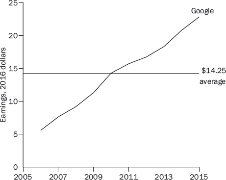
As I noted in valuing Apple, Shiller’s cyclically adjusted P/E ratio (CAPE) can be misleading for companies that have been growing very rapidly. Google’s earnings had been increasing at an annual rate of 33 percent over the past ten years and 14 percent over the past five years, and Figure 13-5 shows that Google’s $14.25 average earnings per share during the years 2006 through 2015 surely understates Google’s current and projected future earnings. (Google’s earnings were $22.84 in 2015 and predicted to be $28.00 in 2016.)

Nonetheless, I calculated Google’s cyclically adjusted earnings yield (CAEP) by dividing its average inflation-adjusted earnings by its inflation adjusted stock price.

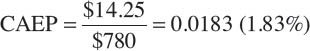
Since this 1.83 percent earnings yield is a rough estimate of a stock’s real rate of return, I compared Google’s CAEP to the real interest rate on ten-year Treasury bonds.

Table 13-5 shows the calculations, using an assumed 2.5 percent rate of inflation. Google was less attractive than the overall S&P 500 by this metric, but there was still a 2.50 percentage-point difference between the Google’s cyclically adjusted earnings yield and the real return on ten-year Treasury bonds.

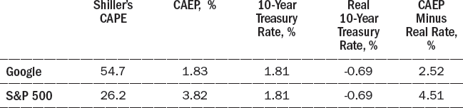
Taking into account the fact that $14.25 is a conservative number for Google’s earnings, its stock becomes more attractive. A line fit to Google’s earnings is so close to actual earnings as to be barely distinguishable. This fitted line implies 2015 cyclically adjusted earnings of $22.73, which increases Google’s CAEP and projected real return to 2.91 percent, which is 3.60 percent above the projected real return on ten-year Treasury bonds.

Now, let’s use John Bogle’s model for estimating Google stock returns over a ten-year horizon:

Google’s price-earnings ratio was 28 in August 2016, somewhat above the S&P 500 P/E of 24. Table 13-6 shows the returns predicted by the Bogle model for the assumption that Google and S&P 500 earnings grow by 5 percent a year and that the price-earnings ratios in ten years (2026) are still 28 for Google and 24 for the S&P 500. Table 13-6 also shows the total returns if Google’s earnings grow by 10 percent a year for the next ten years, and if Google and the S&P 500 both have a P/E of 20 in 2026. Since both P/Es would be going down, this reduces the ten-year annual return on both.

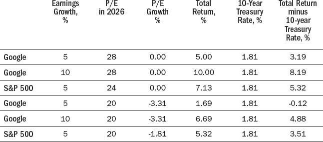
One of the appealing features of the Bogle model is that the calculations can be done in your head or on the back of an envelope. Google does not pay dividends, so the return is solely from the price appreciation over the next ten years. (If Google did pay dividends, we would simply add the dividend yield to the annual price appreciation.)

Google’s projected price appreciation is due to the projected annual rate of increase in its earnings and the change (if any) in its price-earnings ratio. If the P/E is unchanged, then Google’s annual price appreciation will be 5 percent, if its earnings grow by 5 percent, and 10 percent if its earnings grow by 10 percent. If Google’s P/E goes up or down by, say, one percent a year, the projected return goes down or up by the same amount.

Table 13-7 summarizes my calculations for the Shiller and Bogle models. I concluded that the case for Google was not as compelling as the case for Apple, but I thought Google was more attractive than the overall S&P 500 because:

1.I expected Google’s earnings to increase by at least 10 percent annually over the next ten years.

2.I thought it was unlikely that Google’s P/E in 2026 would be less than that for the S&P 500.

I had a substantial holding of Google stock in August 2016, though not nearly as large as my Apple holdings.

	Total Return Minus Treasury Rate, %
SHILLER MODEL
Google, with CAEP = 1.83%	2.52
Google, with CAEP = 2.91%	3.60
S&P 500, with CAEP = 3.82%	4.51
BOGLE MODEL
Google, with 5% earnings growth and P/E = 28 in 2026	3.19
Google, with 10% earnings growth and P/E = 28 in 2026	8.19
S&P 500, with 5% earnings growth and P/E = 24 in 2026	5.32
Google, with 5% earnings growth and P/E = 20 in 2026	–0.12
Google, with 10% earnings growth and P/E = 20 in 2026	4.88
S&P 500, with 5% earnings growth and P/E = 20 in 2026	3.51

AMAZON

I was on sabbatical during the 2015–2016 academic year. As part of my transition back to teaching, I decided to get a new briefcase. My current briefcase had lasted thirty years and its beaten-down charm had morphed into beaten-down raggedy. My wife and children made faces, so I searched Amazon, found a briefcase I liked, and ordered it. With Amazon Prime, the shipping was fast and free.

When I opened the box, my wife and our four children made faces again. I shipped the briefcase back at Amazon’s expense and my wife picked out a briefcase she liked. The shipping was fast and free, and so was the return when I found out that it was too small. It took three more tries before we found a briefcase that everyone liked. Yes, the time needed to reach a decision is proportional to the square of the number of people involved.

How can Amazon afford free shipping both ways? It can’t. Amazon Prime costs $99 a year and includes free two-day shipping (same-day delivery in some places), free streaming of movies, television shows, music, and ebooks. Most returns are free, too.

Amazon sells more than $100 billion of stuff annually to 250 million active users, including more than 50 million Amazon Prime members, but it barely makes a profit. Some years, it loses money. It lost $241 million in 2014, but bounced back with a $596 million profit in 2015. Even the $596 million profit was only a razor-thin 0.55 percent on its 2015 revenue of $107 billion.

Amazon was founded by Jeff Bezos, whose mom was a teenager when he was born and whose stepfather was a Cuban refugee. He got bachelor of science degrees from Princeton in electrical engineering and computer science. Bright and tireless, he worked on Wall Street and then set out to conquer the retail world with Amazon. And conquer it he has.

Scalable technology is technology that allows a business to grow with very little incremental cost. If your business model is making necklaces by hand, the cost of making the thousandth necklace is about the same as the cost of making the first one. If your business model is making a downloadable app, the cost of getting the app to the thousandth customer is much less than the cost of creating the app for the first customer. If your business model is a web page that sells advice, the cost of selling advice to the thousandth customer is much less than the cost of setting up the page to sell advice to the first customer.

Scalability can create a winner-take-all market. If the cost of creating the product is huge and the cost of selling additional products is trivial, the initial cost creates an effective barrier to entry and the small cost of selling additional products allows an established firm with lots of customers to undercut the prices of new entrants. This is the rationale for the commonplace rule in Silicon Valley: “Growth first, revenue later.” Big companies scare away competitors and undercut those who dare to compete. Once a company is established as the biggest, cheapest, and best known, it can collect monopolistic profits.

Amazon’s strategy has been growth first. However, Amazon is no longer a start-up. It is a dominant company that should be ready to reap the rewards of a monopoly, yet every success seems to fund ever more ambitious projects: phones, tablets, one-hour delivery service, movies, cloud computing. Amazon is a terrific company, but where are the profits?

Amazon does not pay dividends, so, as with Google, I can’t use the dividend-discount model and John Burr Williams (JBW) equation. Instead, I used the Shiller and Bogle models.

Figure 13-6 shows that, unlike Apple and Google, Amazon’s earnings have not been growing rapidly. Indeed, the biggest investor complaint about Amazon is that it keeps spending money in order to get bigger and do more things—which leaves shareholders wishing that Amazon would use its market domination to earn some profits. Amazon’s earnings have fallen by 4 percent a year over the past ten years and by 26 percent a year over the past five years.

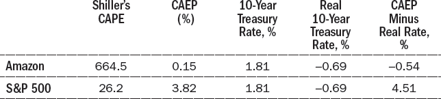
As with Apple and Google, I calculated Amazon’s cyclically adjusted earnings yield (CAEP) and compared it to the real interest rate on ten-year Treasury bonds. Table 13-8 shows the calculations, using an assumed 2.5 percent rate of inflation. Amazon’s cyclically adjusted price-earnings ratio is a mind-boggling 664.5, and its CAEP is a minuscule 0.15 percent (yep, fifteen-hundreds of one percent). By this measure, Amazon is not only less attractive than the S&P 500, its projected return is less than that on ten-year Treasury bonds.

John Bogle’s model for estimating stock returns over a ten-year horizon is

Amazon’s price-earnings ratio was a dizzying 600 in August 2016. I’m acrophobic when it comes to stocks, and a P/E of 600 terrifies me, as it should all value investors. Table 13-9 shows the returns predicted by the Bogle model for the assumption that the price-earnings ratios in 2026 are still 600 for Amazon and 24 for the S&P 500, and that both earnings grow at 5 percent annually. Table 13-9 also shows the total returns if Amazon’s earnings grow by 10 percent a year for the next ten years, and if Amazon and the S&P 500 both have a P/E of 20 in 2026.

Table 13-10 summarizes the calculations for the Shiller and Bogle models. I concluded that Amazon was too risky for my tastes. Its P/E cannot defy gravity forever. Perhaps Amazon’s earnings will soar, which, by itself, will reduce the price-earnings ratio. But an increase in earnings with no dividends and the stock price unchanged doesn’t give investors anything. Or maybe Amazon’s P/E will fall because Amazon’s stock price collapses, which is even worse for investors.

I love Amazon, but I don’t like the stock. Its earnings may explode, but it is too perilous an investment for me.

	Total Return Minus Treasury Rate, %
SHILLER MODEL
Amazon, with CAEP = 0.15%	–0.54
S&P 500, with CAEP = 3.82%	4.51
BOGLE MODEL
Amazon, with 5% earnings growth and P/E = 600 in 2026	3.19
Amazon, with 10% earnings growth and P/E = 600 in 2026	8.19
S&P 500, with 5% earnings growth and P/E = 24 in 2026	5.32
Amazon, with 5% earnings growth and P/E = 20 in 2026	22.02
Amazon, with 10% earnings growth and P/E = 20 in 2026	–17.02
S&P 500, with 5% earnings growth and P/E = 20 in 2026	3.51