Getting straight to the point, the explain method will give us statistics from the query execution. For instance, we will see in these statistics whether a cursor is used or an index.

Let's use the following products collection as an example:

{
   "_id": ObjectId("54bee5c49a5bc523007bb779"),
   "name": "Product 1",
   "price": 56
}
{
   "_id": ObjectId("54bee5c49a5bc523007bb77a"),
   "name": "Product 2",
   "price": 64
}
{
   "_id": ObjectId("54bee5c49a5bc523007bb77b"),
   "name": "Product 3",
   "price": 53
}
{
   "_id": ObjectId("54bee5c49a5bc523007bb77c"),
   "name": "Product 4",
   "price": 50
}
{
   "_id": ObjectId("54bee5c49a5bc523007bb77d"),
   "name": "Product 5",
   "price": 89
}
{
   "_id": ObjectId("54bee5c49a5bc523007bb77e"),
   "name": "Product 6",
   "price": 69
}
{
   "_id": ObjectId("54bee5c49a5bc523007bb77f"),
   "name": "Product 7",
   "price": 71
}
{
   "_id": ObjectId("54bee5c49a5bc523007bb780"),
   "name": "Product 8",
   "price": 40
}
{
   "_id": ObjectId("54bee5c49a5bc523007bb781"),
   "name": "Product 9",
   "price": 41
}
{
   "_id": ObjectId("54bee5c49a5bc523007bb782"),
   "name": "Product 10",
   "price": 53
}

As we have already seen, when the collection is created, an index in the _id field is added automatically. To get all the documents in the collection, we will execute the following query in the mongod shell:

db.products.find({price: {$gt: 65}})

The result of the query will be the following:

{
   "_id": ObjectId("54bee5c49a5bc523007bb77d"),
   "name": "Product 5",
   "price": 89
}
{
   "_id": ObjectId("54bee5c49a5bc523007bb77e"),
   "name": "Product 6",
   "price": 69
}
{
   "_id": ObjectId("54bee5c49a5bc523007bb77f"),
   "name": "Product 7",
   "price": 71
}

To help you understand how MongoDB reaches this result, let's use the explain method on the cursor that was returned by the command find:

db.products.find({price: {$gt: 65}}).explain("executionStats")

The result of this operation is a document with information about the selected query plan:

{
   "queryPlanner" : {
      "plannerVersion" : 1,
      "namespace" : "ecommerce.products",
      "indexFilterSet" : false,
      "parsedQuery" : {
         "price" : {
            "$gt" : 65
         }
      },
      "winningPlan" : {
         "stage" : "COLLSCAN",
         "filter" : {
            "price" : {
               "$gt" : 65
            }
         },
         "direction" : "forward"
      },
      "rejectedPlans" : [ ]
   },
   "executionStats" : {
      "executionSuccess" : true,
      "nReturned" : 3,
      "executionTimeMillis" : 0,
      "totalKeysExamined" : 0,
      "totalDocsExamined" : 10,
      "executionStages" : {
         "stage" : "COLLSCAN",
         "filter" : {
            "price" : {
               "$gt" : 65
            }
         },
         "nReturned" : 3,
         "executionTimeMillisEstimate" : 0,
         "works" : 12,
         "advanced" : 3,
         "needTime" : 8,
         "needFetch" : 0,
         "saveState" : 0,
         "restoreState" : 0,
         "isEOF" : 1,
         "invalidates" : 0,
         "direction" : "forward",
         "docsExamined" : 10
      }
   },
   "serverInfo" : {
      "host" : "c516b8098f92",
      "port" : 27017,
      "version" : "3.0.2",
      "gitVersion" : "6201872043ecbbc0a4cc169b5482dcf385fc464f"
   },
   "ok" : 1
}

Initially, let's check only four fields in this document: queryPlanner.winningPlan.stage, queryPlanner.executionStats.nReturned, queryPlanner.executionStats.totalKeysExamined, and queryPlanner.executionStats.totalDocsExamined:

What happens if we create an index of the price field of our collection? Let's see:

db.products.createIndex({price: 1})

Obviously, the query result will be the same three documents that were returned in the previous execution. However, the result for the explain command will be the following:

{
   "queryPlanner" : {
      "plannerVersion" : 1,
      "namespace" : "ecommerce.products",
      "indexFilterSet" : false,
      "parsedQuery" : {
         …
      },
      "winningPlan" : {
         "stage" : "FETCH",
         "inputStage" : {
            "stage" : "IXSCAN",
            "keyPattern" : {
               "price" : 1
            },
            "indexName" : "price_1",
            ...
         }
      },
      "rejectedPlans" : [ ]
   },
   "executionStats" : {
      "executionSuccess" : true,
      "nReturned" : 3,
      "executionTimeMillis" : 20,
      "totalKeysExamined" : 3,
      "totalDocsExamined" : 3,
      "executionStages" : {
         "stage" : "FETCH",
         "nReturned" : 3,
         ...
         "inputStage" : {
            "stage" : "IXSCAN",
            "nReturned" : 3,
            ...
         }
      }
   },
   "serverInfo" : {
      ...
   },
   "ok" : 1
}

The returned document is fairly different from the previous one. Once again, let's focus on these four fields: queryPlanner.winningPlan.stage, queryPlanner.executionStats.nReturned, queryPlanner.executionStats.totalKeysExamined, and queryPlanner.executionStats.totalDocsExamined.

This time, we can see that we did not have a full collection scan. Instead of this, we had a FETCH stage with a child IXSCAN stage, as we can see in the queryPlanner.winningPlan.inputStage.stage field. This means that the query used an index. The name of the index can be found in the field queryPlanner.winningPlan.inputStage.indexName, in the example, price_1.

Furthermore, the mean difference in this result is that both queryPlanner.executionStats.totalDocsExamined and queryPlanner.executionStats.totalKeysExamined, returned the value 3, showing us that three documents were scanned. It is quite different from the 10 documents that we saw when executing the query without an index.

One point we should make is that the number of documents and keys scanned is the same as we can see in queryPlanner.executionStats.totalDocsExamined and queryPlanner.executionStats.totalKeysExamined. This means that our query was not covered by the index. In the next section, we will see how to cover a query using an index and what its benefits are.

Sometimes we can choose to create indexes with one or more fields, considering the frequency that they appear in our queries. We can also choose to create indexes in order to improve query performance, using them not only to match the criteria but also to extract results from the index itself.

We may say that, when we have a query, all the fields in the criteria are part of an index and when all the fields in the query are part of the same index, this query is covered by the index.

In the example shown in the previous section, we had an index created of the price field of the products collection:

db.products.createIndex({price: 1})

When we execute the following query, which retrieves the documents where the price field has a value greater than 65 but with a projection where we excluded the _id field from the result and included only the price field, we will have a different result from the one previously shown:

db.products.find({price: {$gt: 65}}, {price: 1, _id: 0})

The result will be:

{ "price" : 69 }
{ "price" : 71 }
{ "price" : 89 }

Then we analyze the query using the explain command, as follows:

db.products.explain("executionStats")
.find({price: {$gt: 65}}, {price: 1, _id: 0})

By doing this, we also have a different result from the previous example:

{
   "queryPlanner" : {
      "plannerVersion" : 1,
      "namespace" : "ecommerce.products",
      "indexFilterSet" : false,
      "parsedQuery" : {
         "price" : {
            "$gt" : 65
         }
      },
      "winningPlan" : {
         "stage" : "PROJECTION",
         ...
         "inputStage" : {
            "stage" : "IXSCAN",
            ...

         }
      },
      "rejectedPlans" : [ ]
   },
   "executionStats" : {
      "executionSuccess" : true,
      "nReturned" : 3,
      "executionTimeMillis" : 0,
      "totalKeysExamined" : 3,
      "totalDocsExamined" : 0,
      "executionStages" : {
         ...
      }
   },
   "serverInfo" : {
      ...
   },
   "ok" : 1
}

The first thing we notice is that the value of queryPlanner.executionStats.totalDocsExamined is 0. This can be explained because our query is covered by the index. This means that we do not need to scan the documents from the collection. We will use the index to return the results, as we can observe in the value 3 for the queryPlanner.executionStats.totalKeysExamined field.

Another difference is that the IXSCAN stage is not a child of the FETCH stage. Every time that an index covers a query, IXSCAN will not be a descendent of the FETCH stage.

Unfortunately, it's not always the case that we will have a query covered, even though we had the same conditions that were described previously.

Considering the following customers collection:

{
   "_id": ObjectId("54bf0d719a5bc523007bb78f"),
   "username": "customer1",
   "email": "[email protected]",
   "password": "1185031ff57bfdaae7812dd705383c74",
   "followedSellers": [
       "seller3",
       "seller1"
   ]
}
{
   "_id": ObjectId("54bf0d719a5bc523007bb790"),
   "username": "customer2",
   "email": "[email protected]",
   "password": "6362e1832398e7d8e83d3582a3b0c1ef",
   "followedSellers": [
      "seller2",
      "seller4"
   ]
}
{
   "_id": ObjectId("54bf0d719a5bc523007bb791"),
   "username": "customer3",
   "email": "[email protected]",
   "password": "f2394e387b49e2fdda1b4c8a6c58ae4b",
   "followedSellers": [
      "seller2",
      "seller4"
   ]
}
{
   "_id": ObjectId("54bf0d719a5bc523007bb792"),
   "username": "customer4",
   "email": "[email protected]",
   "password": "10619c6751a0169653355bb92119822a",
   "followedSellers": [
      "seller1",
      "seller2"
   ]
}
{
   "_id": ObjectId("54bf0d719a5bc523007bb793"),
   "username": "customer5",
   "email": "[email protected]",
   "password": "30c25cf1d31cbccbd2d7f2100ffbc6b5",
   "followedSellers": [
      "seller2",
      "seller4"
   ]
}

And an index created of the followedSellers field, executing the following command on mongod shell:

db.customers.createIndex({followedSellers: 1})

If we execute the following query on mongod shell, which was supposed to be covered by the index, since we are using followedSellers on the query criteria:

db.customers.find(
{
   followedSellers: {
      $in : ["seller1", "seller3"]
   }
}, 
{followedSellers: 1, _id: 0}
)

When we analyze this query using the explain command on the mongod shell, to see if the query is covered by the index, we can observe:

db.customers.explain("executionStats").find(
{
   followedSellers: {
      $in : ["seller1", "seller3"]
   }
}, 
{followedSellers: 1, _id: 0}
)

We have the following document as a result. We can see that, despite using a field that is in the index in the criteria and restricting the result to this field, the returned output has the FETCH stage as a parent of the IXSCAN stage. In addition, the values for totalDocsExamined and totalKeysExamined are different:

{
   "queryPlanner" : {
      "plannerVersion" : 1,
      "namespace" : "ecommerce.customers",
      ...
      "winningPlan" : {
         "stage" : "PROJECTION",
         ...
         "inputStage" : {
            "stage" : "FETCH",
            "inputStage" : {
               "stage" : "IXSCAN",
               "keyPattern" : {
                  "followedSellers" : 1
               },
               "indexName" : "followedSellers_1",
               ...
            }
         }
      },
      "rejectedPlans" : [ ]
   },
   "executionStats" : {
      "executionSuccess" : true,
      "nReturned" : 2,
      "executionTimeMillis" : 0,
      "totalKeysExamined" : 4,
      "totalDocsExamined" : 2,
      "executionStages" : {
      ...
      }
   },
   "serverInfo" : {
      ...
},
   "ok" : 1
}

The totalDocsExamined field returned 2, which means that it was necessary to scan two of the five documents from the collection. Meanwhile, the totalKeysExamined field returned 4, showing that it was necessary to scan four index entries for the returned result.

Another situation in which we do not have the query covered by an index is when the query execution is used in an index of a field that is part of an embedded document.

Let's check the example using the products collection that was already used in Chapter 4, Indexing, with an index of the supplier.name field:

db.products.createIndex({"supplier.name": 1})

The following query will not be covered by the index:

db.products.find(
   {"supplier.name": "Supplier 1"}, 
   {"supplier.name": 1, _id: 0}
)

Finally, when we are executing a query in a sharded collection, through mongos, this query will never be covered by an index.

Now that you understand both evaluating query performance using the explain() method and how to take advantage of an index by covering a query, we will proceed to meet the huge responsibility of selecting and maintaining the query plan in MongoDB, the query optimizer.

The query optimizer is responsible for processing and selecting the best and most efficient query plan for a query. For this purpose, it takes into account all the collection indexes.

The process performed by the query optimizer is not an exact science, meaning that it is a little bit empirical—in other words, based on trial and error.

When we execute a query for the very first time, the query optimizer will run the query against all available indexes of the collection and choose the most efficient one. Thereafter, every time we run the same query or queries with the same pattern, the selected index will be used for the query plan.

Using the same products collection we used previously in this chapter, the following queries will run through the same query plan because they have the same pattern:

db.products.find({name: 'Product 1'})
db.products.find({name: 'Product 5'})

As the collection's data changes, the query optimizer re-evaluates it. Moreover, as the collection grows (more precisely for each 1,000 write operations, during each index creation, when the mongod process restarts, or when we call the explain() method), the optimizer re-evaluates itself.

Even with this marvelous automatic process known as the query optimizer, we may want to choose which index we want to use. For this, we use the hint method.

Suppose that we have these indexes in our previous products collection:

db.products.createIndex({name: 1, price: -1})
db.products.createIndex({price: -1})

If we want to retrieve all the products where the price field has a value greater than 10, sorted by the name field in descending order, use the following command to do this:

db.products.find({price: {$gt: 10}}).sort({name: -1})

The index chosen by the query optimizer will be the one created on the name and price fields, as we could see running the explain() method:

db.products.explain("executionStats").find({price: {$gt: 10}}).sort({name: -1})

The result is:

{
   "queryPlanner" : {
      "plannerVersion" : 1,
      "namespace" : "ecommerce.products",
      ...
      "winningPlan" : {
         "stage" : "FETCH",
         ...
         "inputStage" : {
            "stage" : "IXSCAN",
            "keyPattern" : {
               "name" : 1,
               "price" : -1
            },
            "indexName" : "name_1_price_-1"
         ...
         }
      },
      ...
   },
   "executionStats" : {
      "executionSuccess" : true,
      "nReturned" : 10,
      "executionTimeMillis" : 0,
      "totalKeysExamined" : 10,
      "totalDocsExamined" : 10,
      "executionStages" : {
      ...
      }
   },
   "serverInfo" : {
      ...
},
   "ok" : 1
}

However, we can force the use of the index only of the price field, in this manner:

db.products.find(
   {price: {$gt: 10}}
).sort({name: -1}).hint({price: -1})

To be certain, we use the explain method:

db.products.explain("executionStats").find(
   {price: {$gt: 10}}).sort({name: -1}
).hint({price: -1})

This produces the following document:

{
   "queryPlanner" : {
      "plannerVersion" : 1,
      "namespace" : "ecommerce.products",
      ...
      "winningPlan" : {
         "stage" : "SORT",
         ...
         "inputStage" : {
            "stage" : "KEEP_MUTATIONS",
            "inputStage" : {
               "stage" : "FETCH",
               "inputStage" : {
                  "stage" : "IXSCAN",
                  "keyPattern" : {
                     "price" : -1
                  },
                  "indexName" : "price_-1",
                  ...
               }
            }
         }
      },
      "rejectedPlans" : [ ]
   },
   "executionStats" : {
      "executionSuccess" : true,
      "nReturned" : 10,
      "executionTimeMillis" : 0,
      "totalKeysExamined" : 10,
      "totalDocsExamined" : 10,
      "executionStages" : {
         ...
      }
   },
   "serverInfo" : {
      ...
   },
   "ok" : 1
}

So far, we have spoken a lot about reading from one MongoDB instance. Nevertheless, it is important that we speak briefly about reading from a sharded environment or from a replica set.

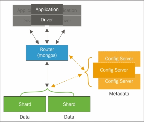
When we are reading from a shard, it is important to have the shard key as part of the query criteria. This is because, when we have the shard key, we will target the execution on one specific shard, whereas if we do not have the shard key, we will force the execution on all the shards in the cluster. Thus, the performance of a query in a sharded environment is linked to the shard key to a great extent.

By default, when we have a replica set in MongoDB, we will always read from the primary. We can modify this behavior to force a read operation execution on to a secondary node by modifying the read preferences.

Suppose that we have a replica set with three nodes: rs1s1, rs1s2, and rs1s3 and that rs1s1 is the primary node, and rs1s2 and rs1s3 are the secondary nodes. To execute a read operation forcing the read on a secondary node, we could do:

db.customers.find().readPref({mode: 'secondary'})

In addition, we have the following read preference options:

In short, if our application wants to maximize consistency, then we should prioritize the read on the primary; when we are looking for availability, we should use primaryPreferred because we can guarantee consistency on most of the reads. When something goes wrong in the primary node, we can count on any secondary node. Finally, if we are looking for the lowest latency, we may use nearest, reminding ourselves that we do not have a guarantee of data consistency because we are prioritizing the lowest latency network node.