, respectively.
from kivy.app import App
from kivy.uix.floatlayout import FloatLayout
from kivy.clock import Clock
from kivy.core.image import Image as CoreImage
from PIL import Image, ImageDraw, ImageFont
import io
import os
import numpy as np
import sympy as sp
from kivy.lang import Builder
Builder.load_file(
os.path.join(os.path.dirname(os.path.abspath(
__file__)), 'File.kv')
);
#import scipy.special as Special
#Avoid Form1 of being resizable
from kivy.config import Config
Config.set("graphics","resizable", False);
Config.set('graphics', 'width', '480');
Config.set('graphics', 'height', '680');
x=sp.symbols("x");
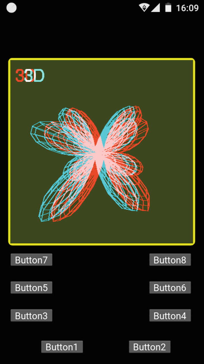
def Plm(l,m ):
N=( 1/(2**l) )*(1 /sp.factorial(l) )
return N * ( (1-x**2)**(m/2) )
* sp.diff( (x**2-1)**l, x,m+l );
R=sp.lambdify( x, Plm(3,2) );
def P2(x):
return 15*x*(1-x**2);
XC=0; YC=0; W=0; H=0;
D=500;
VX1=60; VY1=60; VZ1=0;
VX2=80; VY2=60; VZ2=0;
P=0.5; #Place the function at z=D/2
N=40; #Number of pixels to represent the function
Pi=np.pi;
Theta=np.zeros(N+1); Phi=np.zeros(N+1);
for n in range(0,N+1):
Theta[n]=n/N*Pi;
Phi[n]=n/N*2*Pi;
M_Num=2; N_Num=3; #Legendre m,n orders
F=np.zeros( (N+1,N+1) );
for n in range(0,N+1):
for m in range(0,N+1):
F[n,m]=np.abs( R(np.cos(Theta[n]))
*np.cos(M_Num*Phi[m]) )**2;
x1=np.zeros( (N+1,N+1) );
y=np.zeros( (N+1,N+1) );
z1=np.zeros( (N+1,N+1) );
L=2.4;
for n in range(0,N+1):
for m in range(0,N+1):
x1[n][m]=L*F[n][m]*np.sin(Theta[n])
*np.cos(Phi[m]);
z1[n][m]=L*F [n][m]*np.sin(Theta[n])
*np.sin(Phi[m])+D/2;
y[n][m]=L*F[n][m]*np.cos(Theta[n]);
PointList=np.zeros( (N+1,2) );
def GraphFunction(VX,VY,VZ,Which):
global x1,y, z1, N;
#MaxY=np.max(y)
if (Which==0):
r,g,b = 255, 0, 0; #red Image
Draw=Draw1
else:
r,g,b= 0, 200, 200; #cyan image
Draw=Draw2
for n in range (0,N+1): #Horizontal Lines
for m in range (0,N+1):
Factor=(D-VZ)/(D-z1[n][m]-VZ);
xA=XC+Factor*(x1[n][m]-VX)+VX;
yA=YC-Factor*(y[n][m]-VY)-VY;
PointList[m]=xA,yA;
List=tuple( map(tuple,PointList) );
Draw.line( List, fill=(r,g,b), width=2 );
for n in range (0,N+1): #Vertical Lines
for m in range (0,N+1):
Factor=(D-VZ)/(D-z1[m][n]-VZ);
xA=XC+Factor*(x1[m][n]-VX)+VX;
yA=YC-Factor*(y[m][n]-VY)-VY;
PointList[m]=xA,yA;
List=tuple( map(tuple,PointList) );
Draw.line( List, fill=(r,g,b), width=2 );
Font = ImageFont.truetype('Gargi.ttf', 40)
Draw1.text( (10,10), "3D", fill =
(255,0,0,1), font=Font);
Draw2.text( (30,10), "3D", fill =
(0,255,255,1), font=Font);
def ShowScene(B):
Array1=np.array(PilImage1);
Array2=np.array(PilImage2);
Array3=
Array1 | Array2;
PilImage3=Image.fromarray(Array3);
Memory=io.BytesIO();
PilImage3.save(Memory, format="png");
Memory.seek(0);
ImagePNG=CoreImage(Memory, ext="png");
B.ids.Screen1.texture=ImagePNG.texture;
ImagePNG.remove_from_cache()
Memory.close();
PilImage3.close();
Array1=None;
Array2=None;
Array3=None;
def ClearObjects():
Draw1.rectangle( (0, 0, W-10, H-10), fill=
(60, 70, 30, 1) );
Draw2.rectangle( (0, 0, W-10, H-10), fill=
(60, 70, 30, 1) );
def RotateFunction(B, Sense):
global XG0, ZG0
if Sense==-1:
Theta=np.pi/180*(-4.0);
else:
Theta=np.pi/180*(4.0);
Cos_Theta=np.cos(Theta)
Sin_Theta=np.sin(Theta);
X0=0; Y0=0; Z0=D/2 # Center of rotation
for n in range(0,N+1):
for m in range(0,N+1):
if (B.ids.Button3.state=="down" or
B.ids.Button4.state=="down"):
yP=(y[n][m]-Y0)*Cos_Theta
+ (x1[n][m]-X0)*Sin_Theta + Y0;
xP=-(y[n][m]-Y0)*Sin_Theta
+(x1[n][m]-X0)*Cos_Theta + X0;
y[n][m]=yP;
x1[n][m]=xP;
if (B.ids.Button5.state=="down" or
B.ids.Button6.state=="down"):
yP=(y[n][m]-Y0)*Cos_Theta
+ (z1[n][m]-Z0)*Sin_Theta + Y0;
zP=-(y[n][m]-Y0)*Sin_Theta
+(z1[n][m]-Z0)*Cos_Theta + Z0;
y[n][m]=yP;
z1[n][m]=zP;
if (B.ids.Button7.state=="down" or
B.ids.Button8.state=="down"):
xP=(x1[n][m]-X0)*Cos_Theta
+ (z1[n][m]-Z0)*Sin_Theta + X0;
zP=-(x1[n][m]-X0)*Sin_Theta
+(z1[n][m]-Z0)*Cos_Theta + Z0;
x1[n][m]=xP;
z1[n][m]=zP;
class Form1(FloatLayout):
def __init__(Handle, **kwargs):
super(Form1, Handle).__init__(**kwargs);
Event1=Clock.schedule_once(Handle.Initialize);
def Initialize(B, *args):
global W,H, XC,YC;
global PilImage1,PilImage2, Draw1,Draw2;
#P= Percentage of the D distance
global P, Amplitude;
W,H=B.ids.Screen1.size;
XC=int (W/2)+P/(1-P)*VX1;
YC=int(H/2)-P/(1-P)*VY1;
PilImage1= Image.new('RGB', (W-10, H-10),
(60, 70, 30));
Draw1 = ImageDraw.Draw(PilImage1);
PilImage2= Image.new('RGB', (W-10, H-10),
(60, 70, 30));
Draw2 = ImageDraw.Draw(PilImage2);
Font = ImageFont.truetype('Gargi.ttf', 70)
Draw1.text( (30,200), "3D Images", fill =
(255,0,0,1), font=Font);
Draw2.text( (50,200), "3D Images", fill =
(0,255,255,1), font=Font);
ShowScene(B);
def Button1_Click(B):
global Draw1, Draw2;
ClearObjects(); # Clearing Draw1 and Draw2
GraphFunction(VX1,VY1,VZ1,0);
GraphFunction(VX2,VY2,VZ2,1);
ShowScene(B);
def Button2_Click(B):
ClearObjects(); # Clearing Draw1 and Draw2
Font = ImageFont.truetype('Gargi.ttf', 70)
Draw1.text( (30,200), "3D Images", fill =
(255,0,0,1), font=Font);
Draw2.text( (50,200), "3D Images", fill =
(0,255,255,1), font=Font);
ShowScene(B);
def Button3_Click(B):
RotateFunction(B,1);
ClearObjects(); # Clearing Draw1 and Draw2
GraphFunction(VX1,VY1,VZ1,0);
GraphFunction(VX2,VY2,VZ2,1);
ShowScene(B);
def Button4_Click(B):
RotateFunction(B,-1),
ClearObjects();
GraphFunction(VX1,VY1,VZ1,0);
GraphFunction(VX2,VY2,VZ2,1);
ShowScene(B);
def Button5_Click(B):
RotateFunction(B,-1),
ClearObjects();
GraphFunction(VX1,VY1,VZ1,0);
GraphFunction(VX2,VY2,VZ2,1);
ShowScene(B);
def Button6_Click(B):
RotateFunction(B,1),
ClearObjects();
GraphFunction(VX1,VY1,VZ1,0);
GraphFunction(VX2,VY2,VZ2,1);
ShowScene(B);
def Button7_Click(B):
RotateFunction(B,-1),
ClearObjects();
GraphFunction(VX1,VY1,VZ1,0);
GraphFunction(VX2,VY2,VZ2,1);
ShowScene(B);
def Button8_Click(B):
RotateFunction(B,1),
ClearObjects();
GraphFunction(VX1,VY1,VZ1,0);
GraphFunction(VX2,VY2,VZ2,1);
ShowScene(B);
# This is the Start Up code
.
class StartUp (App):
def build (BU):
BU.title="Form1"
return Form1();
if __name__ =="__main__":
StartUp().run();
Listing 13-4Code for the main.py File