© The Author(s), under exclusive license to APress Media, LLC, part of Springer Nature 2021
M. Cywiak, D. CywiakMulti-Platform Graphics Programming with Kivyhttps://doi.org/10.1007/978-1-4842-7113-1_15

15. Stereoscopic Cylindrical Coordinates Plotting

Moisés Cywiak1   and David Cywiak2
(1)
Leon, Guanajuato, Mexico
(2)
Queretaro, Mexico
 

In this chapter, we describe elements for plotting stereoscopic 3D cylindrical functions. For this purpose, we focus on the so-called aberrations of optical lenses, also referred to as Seidel aberrations .

Figure 15-1 shows the program running on an Android cell phone with a stereoscopic plot of one of these terms, referred to as spherical aberration.
../images/510726_1_En_15_Chapter/510726_1_En_15_Fig1_HTML.jpg
Figure 15-1

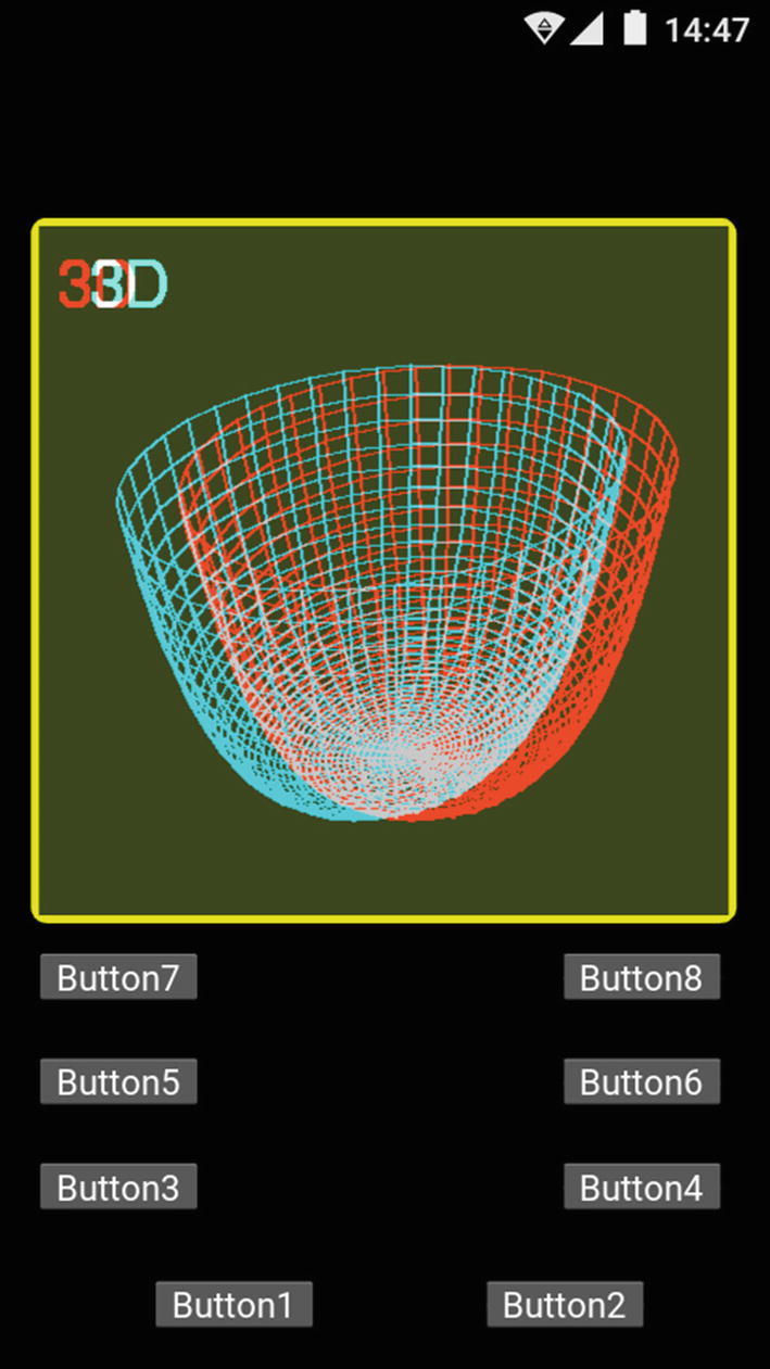
Screenshot of the program on an Android cell phone showing a plot of a spherical aberration term

The functionality of the buttons is the same as in previous chapters.

Seidel aberrations consist of algebraic terms, expressed as typical cylindrical coordinate functions, which can be obtained by expanding the transmittance phase function of an ideal lens by a Taylor series. According to the wave theory of light, in the process of focusing an illuminating light source by a lens, the interaction of the lens with the wavefronts of light prevents the lens from focusing on a single point, generating instead a spatial light distribution around the focal point. A precise analytical tool to calculate the spatial distribution of the focused profiles is given by the Fresnel diffraction integral , which allows one to introduce the concept of the phase transmittance function of a lens. In the next section, we provide an introductory analytical description of this subject.

15.1 Ideal Lens Focusing: The Fresnel Diffraction Integral

In Figure 15-2, an illuminating beam is located at an initial plane with coordinates (x, y). The spatial amplitude distribution of the illuminating beam at the initial plane is represented by ψ(x, y). The light propagates to the right, from plane (x, y) to an observation plane with coordinates (ξ, η), placed at a distance z. The planes are parallel. The amplitude distribution of the propagated field is given by ψF(ξ, η).
../images/510726_1_En_15_Chapter/510726_1_En_15_Fig2_HTML.jpg
Figure 15-2

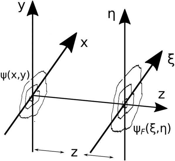
An initial field with amplitude distribution ψ(x, y) propagates a distance z toward an observation plane. The parameter ψF(ξ, η) represents the amplitude distribution at the plane of observation

As mentioned, an accurate tool to calculate the amplitude distribution of the field at the observation plane is given by the Fresnel diffraction integral, expressed as follows:
$$ {psi}_Fleft(xi, eta 
ight)=frac{mathit{exp}left(ifrac{2pi z}{lambda}
ight)}{ilambda z}{int}_{-infty}^{infty }{int}_{-infty}^{infty}psi left(x,y
ight)mathit{exp}left[frac{ipi}{lambda z}left({left(x-xi 
ight)}^{{}^2}+{left(y-eta 
ight)}^{{}^2}
ight)
ight] dx dy $$
(15.1)

For our program, we will apply the Fresnel diffraction integral to the case of an ideal lens. As is well known, a physical property that characterizes an ideal lens is its capability of focusing a spatially unlimited plane wave. Therefore, at the plane of observation, the focused light distribution should consist of an ideal geometrical point. Analytically, the corresponding equation of this point at the plane of observation is represented as δ(ξ, η). Here the δ symbol represents a Dirac delta function.

In Equation (15.1), we use the following substitution:
$$ psi left(x,y
ight)=mathit{exp}left(-frac{ipi}{lambda f}left({x}^{{}^2}+{y}^{{}^2}
ight)
ight) $$
(15.2)

In Equation (15.2), ψ(x, y) represents the transmittance function of the ideal lens. In the exponential function with an imaginary argument, the quadratic expression is referred to as the phase of the lens. We will now see that this quadratic negative phase results in a convergent wavefront.

Substituting Equation (15.2) into Equation (15.1) gives the following equation:
$$ {psi}_Fleft(xi, eta 
ight)=frac{mathit{exp}left(ifrac{2pi f}{lambda}
ight)}{ilambda f}{int}_{-infty}^{infty }{int}_{-infty}^{infty}mathit{exp}left(-frac{ipi}{lambda f}left({x}^{{}^2}+{y}^{{}^2}
ight)
ight)mathit{exp}left(frac{ipi}{lambda f}left({left(x-xi 
ight)}^{{}^2}+{left(y-eta 
ight)}^{{}^2}
ight)
ight) dx dy $$
(15.3)

In Equation (15.3), we substituted z with f, the lens focal length.

By expanding the binomial terms in the second exponential in the integral of Equation (15.3) and canceling same terms, we get:
$$ {psi}_Fleft(xi, eta 
ight)=frac{mathit{exp}left(ifrac{2pi f}{lambda}
ight)}{ilambda f}mathit{exp}left(frac{ipi}{lambda f}left({xi}^2+{eta}^2
ight)
ight){int}_{-infty}^{infty }{int}_{-infty}^{infty}mathit{exp}left(-frac{i2pi }{lambda f}left( xxi +kern21.5em yeta 
ight)
ight) dx dy $$
(15.4)
In Equation (15.4), we recognize that the integral corresponds to one of the representations found in the mathematical tables for a two-dimensional Dirac delta function; that is:
$$ {int}_{-infty}^{infty }{int}_{-infty}^{infty}mathit{exp}left(-frac{i2pi }{lambda f}left( xxi + yeta 
ight)
ight) dx dy=delta left(frac{xi }{lambda f},frac{eta }{lambda f}
ight) $$
(15.5)
Substituting Equation (15.5) into Equation (15.4) gives the following equation:
$$ {psi}_Fleft(xi, eta 
ight)=frac{mathit{exp}left(ifrac{2pi f}{lambda}
ight)}{ilambda f}mathit{exp}left(frac{ipi}{lambda f}left({xi}^{{}^2}+{eta}^{{}^2}
ight)
ight)delta left(xi, eta 
ight) $$
(15.6)
We now apply the $$ fleft(xi, eta 
ight)delta left(frac{xi }{lambda f},frac{eta }{lambda f}
ight)=fleft(0,0
ight){left(lambda f
ight)}^{{}^2}delta left(xi, eta 
ight) $$ property for λ > 0 and f > 0, which allows us to simplify Equation (15.6) as follows:
$$ {psi}_Fleft(xi, eta 
ight)=- ilambda fexpleft(ifrac{2pi f}{lambda}
ight)delta left(xi, eta 
ight) $$
(15.7)

Equation (15.7) demonstrates that when an ideal lens is illuminated by a plane wave that propagates parallel to the optical axes, the lens concentrates (or focuses) the light precisely at the center of the observation plane. The focusing spot consists of an ideal geometrical point, provided that the plane of observation is placed precisely at a lens focal distance from the initial plane.

15.2 Departure from the Ideal Lens

As properties of real lenses deviate from ideal ones, we must devise a more realistic approach. Let’s add a linear term to the ideal lens phase of Equation (15.2), as follows:
$$ psi left(x,y
ight)=mathit{exp}left(-frac{ipi}{lambda f}left({x}^{{}^2}+{y}^{{}^2}+ ax
ight)
ight) $$
(15.8)

In Equation (15.8), the parameter a represents a constant term.

Substituting Equation (15.8) into Equation (15.1) and calculating the integral gives the following:
$$ {psi}_Fleft(xi, eta 
ight)=- ilambda fexpleft(ifrac{2pi f}{lambda}
ight)mathit{exp}left(ifrac{{pi a}^{{}^2}}{lambda f}
ight)delta left(xi -a
ight)delta left(eta 
ight) $$
(15.9)

Equation (15.9) shows that the focused spot has been shifted from the origin in the x-direction, due to the linear term introduced in Equation (15.8). We conclude that the lens has tilted the wavefront with respect to the optical axes. An analog analysis applies to the y-direction.

This approach can be made more general by replacing the phase of the lens by a transmittance function, as follows:
$$ psi left(x,y
ight)=mathit{exp}left( iphi left(x,y
ight)
ight) $$
(15.10)
Now, based on the experience gain in our example, we will assume that the phase function in Equation (15.10) depends on the combination of three independent variables:
$$ phi left(x,y
ight)=phi left({x}^{{}^2}+{y}^{{}^2},{a}^{{}^2}, ax
ight) $$
(15.11)
Equation (15.11) can now be expanded in a similar manner to a Taylor series:
$$ phi left({x}^{{}^2}+{y}^{{}^2},{a}^{{}^2}, ax
ight)={A}_{0,0,0}+{A}_{1,0,0}left({x}^{{}^2}+{y}^{{}^2}
ight)+{A}_{0,1,0}{a}^{{}^2}+{A}_{0,0,1} ax+{A}_{2,0,0}{left({x}^{{}^2}+{y}^{{}^2}
ight)}^{{}^2}+{A}_{0,2,0}{left({a}^{{}^2}
ight)}^{{}^2}+{A}_{0,0,2}{(ax)}^{{}^2}+{A}_{1,1,0}left({x}^{{}^2}+{y}^{{}^2}
ight){a}^{{}^2}+{A}_{1,0,1}left({x}^{{}^2}+{y}^{{}^2}
ight)(ax)+{A}_{0,1,1}left({a}^{{}^2}
ight)(ax)+cdots $$
(15.12)

In Equation (15.12), each coefficient in the series has three sub-indexes. Each sub-index corresponds to the power of its corresponding expansion term. The first sub-index corresponds to the power of the term (x² + y²). The second sub-index corresponds to the power of a². Finally, the third sub-index corresponds to the power of ax. For example, A1, 0, 1 is the coefficient of the term of the products of (x² + y²)¹ by (a²)0 by (ax)¹.

15.3 The Wave Aberration Function in Cylindrical Coordinates

Equation (15.12) is one of the possible expansions of an aberrated wavefront. An algebraic sum of these terms can represent a real lens. Due to circular symmetry in the lens-manufacturing process, the expansion may fit better for analytical lens modeling if the expansion is expressed in cylindrical coordinates. Then, we express x and y as follows:
$$ x=
ho cosleft(	heta 
ight);y=
ho sinleft(	heta 
ight) $$
(15.13)

In Equation (15.13) the variables ρ and θ are, as usual, the radial and polar coordinates, respectively.

Substituting Equation (15.13) into Equation (15.12) gives the following:
$$ phi left({
ho}^{{}^2},{a}^{{}^2}, a
ho cosleft(	heta 
ight)
ight)={A}_{0,0,0}+{A}_{1,0,0}left({
ho}^{{}^2}
ight)+{A}_{0,1,0}{a}^{{}^2}+{A}_{0,0,1} a
ho cosleft(	heta 
ight)+{A}_{2,0,0}{left({
ho}^{{}^2}
ight)}^{{}^2}+{A}_{0,2,0}{left({a}^{{}^2}
ight)}^{{}^2}+{A}_{0,0,2}{left( a
ho cosleft(	heta 
ight)
ight)}^{{}^2}+{A}_{1,1,0}left({
ho}^{{}^2}
ight){a}^{{}^2}+{A}_{1,0,1}left({
ho}^{{}^2}
ight)left( a
ho cosleft(	heta 
ight)
ight)+{A}_{0,1,1}left({a}^{{}^2}
ight)left( a
ho cosleft(	heta 
ight)
ight)+cdots $$
(15.14)

Note that there are other possible expressions for the coefficients.

Table 15-1 gives a brief listing of common names for the aberration terms in Equation (15.14).
Table 15-1

Definition of Some Aberration Terms

Coefficient

Term

Typical Name

A1, 0, 0

ρ²

Focus

A0, 1, 0

a²

Piston

A0, 0, 1

aρcos(θ)

Tilt

A2, 0, 0

(ρ²)²

Spherical

A0, 2, 0

(a²)²

Piston

A0, 0, 2

(aρcos(θ))²

Astigmatism

A1, 1, 0

ρ²a²

Field curvature

A1, 0, 1

ρ²(aρcos(θ))

Coma

A0, 1, 1

a²(aρcos(θ))

Distortion

In the following section, we describe the program that will stereoscopically plot the aberration terms in cylindrical coordinates.

15.4 Stereoscopic Plot of Wave Aberration Terms in Cylindrical Coordinates

As in previous chapters, we need two points of projection to create two images slightly shifted horizontally. The following code sets the coordinates of the projecting points. As in our previous examples, D is the distance between the plane of projection and the screen.
D=800;
VX1=100; VY1=200; VZ1=0;
VX2=130; VY2=200; VZ2=0;

We will place the plot of the aberration terms at the middle between the plane of projection and the screen, using the percentage variable P with a value of 0.5.

Next, we set the number of pixels for the plot and create the mesh, as shown in Listing 15-1.
import numpy as np
N=40;  # Number of pixels to represent the function
y=np.zeros( (N+1,N+1) );
# Creating Mesh array
x1=np.zeros( (N+1,N+1) ); z1=np.zeros( (N+1,N+1) );
Listing 15-1

Creating the Mesh

As in previous chapters, the vertical heights are represented by the y-coordinate; x represents the horizontal coordinate and z represents the depth.

Now we create the radial. and polar coordinates using the code in Listing 15-2.
Pi=np.pi;
Rho=np.zeros(N+1); Theta=np.zeros(N+1);
for n in range(0,N+1):
    Rho[n]=n/N;
    Theta[n]=n/N*2*Pi;
Listing 15-2

Creating and Filling the Radial and Polar Coordinates

The size of both arrays is N+1. The radial array, Rho, has N+1 entries, with entries ranging from 0 to 1. The polar array, Theta, stores values from 0 to 2π.

To control the sizes of the width and depth of the plots, we will define a scaling factor, L.
L=70; # Horizontal and depth scale factor.
Now, we set D equal to 800, which is the distance between the plane of projection and the screen. We also set the percentage value P to 0.5.
D=800;
P=0.5; #Place the function at z=D/2
Now we can create the mesh in the x-z plane with the code shown in Listing 15-3.
ZG0=P*D;
for n in range (0,N+1):
    for m in range(0,N+1):#Filling Mesh
        x1[n][m]=L*Rho[n]*np.cos(Theta[m]);
        z1[n][m]=L*Rho[n]*np.sin(Theta[m])+ZG0;
Listing 15-3

Creating the Mesh in the x-z Plane

We will also define a vertical scaling amplitude for y, as follows:
Amplitude=100; # Vertical scale factor.
Now we can fill the vertical array with data of one of the aberration terms. In the example in Listing 15-4, we use the term that corresponds to spherical aberration.
for n in range(0,N+1): #Filling function pixels
    for m in range(0,N+1):
        # Spherical aberration
        y[n][m]=Amplitude * Rho[n]**4;
Listing 15-4

Filling the Vertical Array

In this code, the spherical aberration term is independent of Theta. For an aberration term depending on Theta, such as tilt for example, the code would be as follows:
for n in range(0,N+1): # Filling function pixels
    for m in range(0,N+1):
        # Tilt
        y[n][m]=Amplitude * Rho[n]*np.cos(Theta[m]);
The remaining functions of the program are the same as in previous chapters. The complete code for main.py and File.kv are shown in Listing 15-5 and Listing 15-6, respectively.
from kivy.app import App
from kivy.uix.floatlayout import FloatLayout
from kivy.graphics import Line, Ellipse, Color
from kivy.clock import Clock
from kivy.core.image import Image as CoreImage
from PIL import Image, ImageDraw, ImageFont
import io
import os
import numpy as np
from kivy.lang import Builder
Builder.load_file(
    os.path.join(os.path.dirname(os.path.abspath(
                        __file__)), 'File.kv')
                  );
# Avoid Form1 of being resizable
from kivy.config import Config
Config.set("graphics","resizable", False);
Config.set('graphics', 'width',  '480');
Config.set('graphics', 'height', '680');
D=800;
VX1=100; VY1=200; VZ1=0;
VX2=130; VY2=200; VZ2=0;
P=0.5; # Place the function at z=D/2
N=40;  # Number of pixels to represent the function
y=np.zeros( (N+1,N+1) );
# Mesh
x1=np.zeros( (N+1,N+1) ); z1=np.zeros( (N+1,N+1) );
L=70;
Pi=np.pi;
XG0=0; ZG0=P*D; Amplitude=100;
Rho=np.zeros(N+1); Theta=np.zeros(N+1);
for n in range(0,N+1):
    Rho[n]=n/N;
    Theta[n]=n/N*2*Pi;
for n in range (0,N+1):
    for m in range(0,N+1):#Filling Mesh
        x1[n][m]=L*Rho[n]*np.cos(Theta[m]);
        z1[n][m]=L*Rho[n]*np.sin(Theta[m])+ZG0;
for n in range(0,N+1): #Filling function pixels
    for m in range(0,N+1):
        y[n][m]=Amplitude * Rho[n]**4;
PointList=np.zeros( (N+1,2) );
def GraphFunction(VX,VY,VZ,Which):
    global x1,y, z1, N;
    # MaxY=np.max(y)
    if (Which==0):
        r,g,b = 200, 0, 0; #red Image
        Draw=Draw1
    else:
        r,g,b= 0, 200, 200; #cyan image
        Draw=Draw2
    for n in range (0,N+1): #Horizontal Lines
        for m in range (0,N+1):
            Factor=(D-VZ)/(D-z1[n][m]-VZ);
            xA=XC+Factor*(x1[n][m]-VX)+VX;
            yA=YC-Factor*(y[n][m]-VY)-VY;
            PointList[m]=xA,yA;
        List=tuple( map(tuple,PointList) );
        Draw.line( List, fill=(r,g,b), width=2 );
    for n in range (0,N+1): #Vertical Lines
        for m in range (0,N+1):
            Factor=(D-VZ)/(D-z1[m][n]-VZ);
            xA=XC+Factor*(x1[m][n]-VX)+VX;
            yA=YC-Factor*(y[m][n]-VY)-VY;
            PointList[m]=xA,yA;
        List=tuple( map(tuple,PointList) );
        Draw.line( List, fill=(r,g,b), width=2 );
        Font = ImageFont.truetype('Gargi.ttf', 40);
        Draw1.text( (10,10), "3D", fill =
                        (255,0,0,1), font=Font);
        Draw2.text( (30,10), "3D", fill =
                        (0,255,255,1), font=Font);
def ShowScene(B):
    Array1=np.array(PilImage1);
    Array2=np.array(PilImage2);
    Array3=Array1 | Array2;
    PilImage3=Image.fromarray(Array3);
    Memory=io.BytesIO();
    PilImage3.save(Memory, format="png");
    Memory.seek(0);
    ImagePNG=CoreImage(Memory, ext="png");
    B.ids.Screen1.texture=ImagePNG.texture;
    ImagePNG.remove_from_cache()
    Memory.close();
    PilImage3.close();
    Array1=None;
    Array2=None;
    Array3=None;
def ClearObjects():
    Draw1.rectangle( (0, 0, W-10, H-10), fill=
                             (60, 70, 30, 1) );
    Draw2.rectangle( (0, 0, W-10, H-10), fill=
                             (60, 70, 30, 1) );
def RotateFunction(B, Sense):
    global XG0, ZG0
    if Sense==-1:
        Teta=np.pi/180*(-4.0);
    else:
        Teta=np.pi/180*(4.0);
    Cos_Teta=np.cos(Teta)
    Sin_Teta=np.sin(Teta);
    X0=XG0;  Y0=0;  Z0=ZG0 # Center of rotation
    for n in range(0,N+1):
        for m in range(0,N+1):
            if (B.ids.Button3.state=="down" or
                        B.ids.Button4.state=="down"):
                yP=(y[n][m]-Y0)*Cos_Teta
                    + (x1[n][m]-X0)*Sin_Teta + Y0;
                xP=-(y[n][m]-Y0)*Sin_Teta
                    +(x1[n][m]-X0)*Cos_Teta + X0;
                y[n][m]=yP;
                x1[n][m]=xP;
            if (B.ids.Button5.state=="down" or
                        B.ids.Button6.state=="down"):
                yP=(y[n][m]-Y0)*Cos_Teta
                    + (z1[n][m]-Z0)*Sin_Teta + Y0;
                zP=-(y[n][m]-Y0)*Sin_Teta
                    +(z1[n][m]-Z0)*Cos_Teta + Z0;
                y[n][m]=yP;
                z1[n][m]=zP;
            if (B.ids.Button7.state=="down" or
                    B.ids.Button8.state=="down"):
                xP=(x1[n][m]-X0)*Cos_Teta
                    + (z1[n][m]-Z0)*Sin_Teta + X0;
                zP=-(x1[n][m]-X0)*Sin_Teta
                    +(z1[n][m]-Z0)*Cos_Teta + Z0;
                x1[n][m]=xP;
                z1[n][m]=zP;
class Form1(FloatLayout):
    def __init__(Handle, **kwargs):
        super(Form1, Handle).__init__(**kwargs);
        Event1=Clock.schedule_once(Handle.Initialize);
    def Initialize(B, *args):
        global W,H, XC,YC;
        global PilImage1,PilImage2, Draw1,Draw2;
        # P= Percentage of the D distance
        global P, Amplitude;
        W,H=B.ids.Screen1.size;
        XC=int (W/2)+P/(1-P)*VX1+30;
        YC=int(H/2)-P/(1-P)*VY1+110;
        PilImage1= Image.new('RGB', (W-10, H-10),
                                 (60, 70, 30));
        Draw1 = ImageDraw.Draw(PilImage1);
        PilImage2= Image.new('RGB', (W-10, H-10),
                                 (60, 70, 30));
        Draw2 = ImageDraw.Draw(PilImage2);
        Font = ImageFont.truetype('Gargi.ttf', 70)
        Draw1.text( (30,200), "3D Images", fill =
                            (255,0,0,1), font=Font);
        Draw2.text( (50,200), "3D Images", fill =
                            (0,255,255,1), font=Font);
        ShowScene(B);
    def Button1_Click(B):
        global Draw1, Draw2;
        ClearObjects(); # Clearing Draw1 and Draw2
        GraphFunction(VX1,VY1,VZ1,0);
        GraphFunction(VX2,VY2,VZ2,1);
        ShowScene(B);
    def Button2_Click(B):
        ClearObjects(); # Clearing Draw1 and Draw2
        Font = ImageFont.truetype('Gargi.ttf', 70)
        Draw1.text( (30,200), "3D Images", fill =
                            (255,0,0,1), font=Font);
        Draw2.text( (50,200), "3D Images", fill =
                          (0,255,255,1), font=Font);
        ShowScene(B);
    def Button3_Click(B):
        RotateFunction(B,1);
        ClearObjects(); # Clearing Draw1 and Draw2
        GraphFunction(VX1,VY1,VZ1,0);
        GraphFunction(VX2,VY2,VZ2,1);
        ShowScene(B);
    def Button4_Click(B):
        RotateFunction(B,-1),
        ClearObjects();
        GraphFunction(VX1,VY1,VZ1,0);
        GraphFunction(VX2,VY2,VZ2,1);
        ShowScene(B);
    def Button5_Click(B):
        RotateFunction(B,-1),
        ClearObjects();
        GraphFunction(VX1,VY1,VZ1,0);
        GraphFunction(VX2,VY2,VZ2,1);
        ShowScene(B);
    def Button6_Click(B):
        RotateFunction(B,1),
        ClearObjects();
        GraphFunction(VX1,VY1,VZ1,0);
        GraphFunction(VX2,VY2,VZ2,1);
        ShowScene(B);
    def Button7_Click(B):
        RotateFunction(B,-1),
        ClearObjects();
        GraphFunction(VX1,VY1,VZ1,0);
        GraphFunction(VX2,VY2,VZ2,1);
        ShowScene(B);
    def Button8_Click(B):
        RotateFunction(B,1),
        ClearObjects();
        GraphFunction(VX1,VY1,VZ1,0);
        GraphFunction(VX2,VY2,VZ2,1);
        ShowScene(B);
# This is the Start Up code.
class StartUp (App):
    def build (BU):
        BU.title="Form1"
        return Form1();
if __name__ =="__main__":
    StartUp().run();
Listing 15-5

Code for the main.py File

#:set W 440
#:set H 440
<Form1>:
    id : Form1
    Image:
        id: Screen1
        size_hint: None,None
        pos_hint: {"x":0.04, "y":0.34}
        size: W,H
        canvas.before:
            Color:
                rgba: 0.9, 0.9, 0, 1
            RoundedRectangle:
                pos:  self.pos
                size: self.size
    Button:
        id: Button1
        on_press: Form1.Button1_Click()
        text: "Button1"
        size_hint: None,None
        pos_hint: {"x": 0.2, "y":0.03}
        size: 100,30
    Button:
        id: Button2
        on_press: Form1.Button2_Click()
        text: "Button2"
        size_hint: None,None
        pos_hint: {"x": 0.63, "y":0.03}
        size: 100,30
    Button:
        id: Button3
        on_press: Form1.Button3_Click()
        text: "Button3"
        size_hint: None,None
        pos_hint: {"x": 0.05, "y":0.12}
        size: 100,30
        always_release: True
    Button:
        id: Button4
        on_press: Form1.Button4_Click()
        text: "Button4"
        size_hint: None,None
        pos_hint: {"x": 0.73, "y":0.12}
        size: 100,30
    Button:
        id: Button5
        on_press: Form1.Button5_Click()
        text: "Button5"
        size_hint: None,None
        pos_hint: {"x": 0.05, "y":0.20}
        size: 100,30
    Button:
        id: Button6
        on_press: Form1.Button6_Click()
        text: "Button6"
        size_hint: None,None
        pos_hint: {"x": 0.73, "y":0.20}
        size: 100,30
    Button:
        id: Button7
        on_press: Form1.Button7_Click()
        text: "Button7"
        size_hint: None,None
        pos_hint: {"x": 0.05, "y":0.28}
        size: 100,30
    Button:
        id: Button8
        on_press: Form1.Button8_Click()
        text: "Button8"
        size_hint: None,None
        pos_hint: {"x": 0.73, "y":0.28}
        size: 100,30
Listing 15-6

Code for the file.kv File

Figure 15-3 shows plots of five aberration terms obtained with the program, corresponding to the coefficients A0, 0, 1, A0, 0, 2, A1, 0, 0, A1, 0, 1, and A2, 0, 0 of Equation (15.12).
../images/510726_1_En_15_Chapter/510726_1_En_15_Fig3_HTML.jpg
Figure 15-3

Wavefront aberration terms corresponding to the coefficients A0, 0, 1, A0, 0, 2, A1, 0, 0, A1, 0, 1, and A2, 0, 0 of Equation (15.12), plotted with the program

15.5 Summary

In this chapter, we introduced elements for plotting stereoscopic 3D cylindrical functions. In particular, we presented working examples of Seidel aberrations. We provided a brief outline of the Fresnel diffraction integral and applied this integral to review the focusing properties of ideal lenses. We extended these concepts to lens aberrations, illustrating programming methods for plotting the aberration terms in stereoscopic views.

..................Content has been hidden....................

You can't read the all page of ebook, please click here login for view all page.
Reset
52.14.126.74