4.1 Projecting a Three-Dimensional Point Onto a Plane

Figure 4-1 depicts two three-dimensional points, P and P^′, with coordinates (x, y, z) and (x^′, y^′, z^′), respectively. Point P^′, the projected point, is obtained by projecting P on the computer’s screen by drawing a straight line from a fixed point V with coordinates (V_X, V_Y, V_Z) up to P^′ and passing through P. Point V is referred to as the point of projection. Vectors P and P^′ correspond to the vectors that go from the origin with coordinates (0, 0, 0) to (x, y, z) and to (x^′, y^′, z^′), respectively.

The unit direction vectors of the three-dimensional space are given by i, j, and k, as depicted in Figure 4-1. For simplicity, the screen is placed parallel to the x − y plane and the normal distance between planes is D.

Let A denote the vector from point V to P and let B denote the vector from point V to P^′. As both vectors are parallel to each other, we can write:

(4.1)

In Equation (4.1), t is a scalar.

It can be seen from Figure 4-1 that:

(4.2)

and:

(4.3)

Using Equations (4.1)-(4.3) gives the following:

(4.4)

On the two-dimensional screen, as depicted in Figure 4-2, the bottom-left corner has coordinates (0, 0), while its center has coordinates (X_C, Y_C). Vector Q corresponds to the vector that goes from (0, 0) to (X_C, Y_C). Vector T goes from (X_C, Y_C) to P^′, while vector R goes from (0, 0) to P^′. As these three vectors are on the screen, each one of them is normal to k.

From Figure 4-2, we can write:

(4.5)

Noticing in Figure 4-1 that the vector Dk goes from (0 ,0, 0) to the center of the screen, we can write:

(4.6)

Using Equations (4.6) and (4.4) gives the following:

(4.7)

Now, as vector T is normal to k, the dot product vanishes. Therefore, the dot product of Equation (4.7) with k gives the following:

(4.8)

Performing the dot products in Equation (4.8) allows us to obtain the following:

(4.9)

To obtain Equation (4.9), we used P = Dk.

Note from Figure 4-1 that z in Equation (4.9) is the distance from the origin (0, 0, 0) to point P, along the unitary k vector. For programming purposes, it is more convenient to measure this distance starting from the screen. This distance is denoted as Z_P. Therefore, z = D − Z_P. This value will be substituted in Equation (4.9).

Now, we use the value of t given by Equation (4.9) and the value of T obtained from Equation (4.5) to rewrite Equation (4.7) as follows:

(4.10)

In Equation (4.10), we substituted z with D − Z_P.

Equation (4.10) allows us to calculate the coordinates of point P^′ on the screen. For this, according to Figure 4-2, we will express vectors R and Q on the screen as R = X_Pi + Y_Pj and Q = X_Ci + Y_Cj. Therefore, Equation (4.10) gives the position of point P^′ in terms of the vector pointing to the center of the screen (Q), the normal distance to the screen (D), the vector of projection (V), and the position of the three-dimensional point (P).

By expressing R = X_Pi + Y_Pj and Q = X_Ci + Y_Cj in Equation (4.10), the vector components give the following three equations:

(4.11)

(4.12)

(4.13)

Equations (4.11) and (4.12) represent the main tool for determining the projection of the three-dimensional point on the screen. Equation (4.13), although algebraically correct, will not be used, as it does not provide further information.

In addition to Equations (4.11) and (4.12), we will also need equations to rotate the polygons. In the following section, we obtain these equations.

4.2 Rotating a Point on a Plane

Rotation equations for a three-dimensional point projected on a screen can be calculated by successive rotations performed in two-dimensional planes. Therefore, our description here is presented in a two-dimensional space.

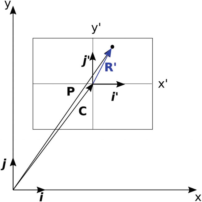
In Figure 4-3, the center of the screen, with coordinates (x^′, y^′), is given by the position vector C on a coordinate plane (x, y).

In Figure 4-3, the black dot represents an arbitrary point on the two-dimensional (x, y) space. As depicted, P and C represent vectors going from the origin of the (x, y) system to the point and to the center of the screen, respectively. Vector R^′ goes from the center of the screen to the point. It can be observed that:

(4.14)

In terms of their components, vectors in Equation (4.14) will be written as follows:

(4.15)

(4.16)

(4.17)

It will also be noticed that:

i = i^′ and j = j^′ (4.18)

We assume that the black dot depicted in Figure 4-3 is fixed on the screen. Therefore, if the screen rotates an angle θ, as illustrated in Figure 4-4, the coordinates of the rotated point remain fixed on the screen.

From Figure 4-4, we obtain the following:

(4.19)

(4.20)

(4.21)

In Equations (4.20) and (4.21), we substituted i^′ and j^′ with their corresponding values given in Equation (4.18).

As mentioned, the rotated point maintains fixed coordinates on the screen; therefore, we can write:

(4.22)

Substituting Equations (4.20) and (4.21) in Equation (4.22) gives the following:

(4.23)

Now, x^′ and y^′ can be calculated using the component vectors of Equation (4.14) as:

(4.24)

(4.25)

By explicitly writing the components of R^′′ in Equation (4.23) and using Equations (4.24) and (4.25), we obtain the following:

(4.26)

(4.27)

Equations (4.26) and (4.27) give the coordinates of the rotated point. These equations are used in Chapter 5 to program the rotation of the polygons.

4.3 Summary

In this chapter, we derived analytical equations for projecting three-dimensional points onto a two-dimensional screen. Additionally, we obtained equations to calculate the rotation of points in a three-dimensional space. These equations are used in Chapter 5 to position and rotate polygons on the screen.