
Demultiplexing
Biologically the species is the accumulation of the experiments of all its successful individuals since the beginning.
— H. G. WELLS
A protocol, like a copy center or an ice cream parlor, should be able to serve multiple clients. The clients of a protocol could be end users (as in the case of the file transfer protocol), software programs (for example, when the tool traceroute uses the Internet protocol), or even other protocols (as in the case of the email protocol SMTP, which uses TCP).
Thus when a message arrives, the receiving protocol must dispatch the received message to the appropriate client. This function is called demultiplexing. Demultiplexing is an integral part of data link, routing, and transport protocols. It is a fundamental part of the abstract protocol model of Chapter 2.
Traditionally, demultiplexing is done layer by layer using a demultiplexing field contained in each layer header of the received message. Called layered demultiplexing, this is shown in Figure 8.1. For example, working from bottom to top in the picture, a packet may arrive on the Ethernet at a workstation. The packet is examined by the Ethernet driver, which looks at a so-called protocol type field to decide what routing protocol (e.g., IP, IPX) is being used. Assuming the type field specifies IP, the Ethernet driver may upcall the IP software.
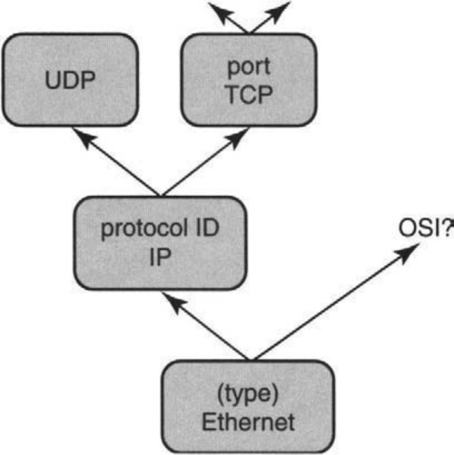
After IP processing, the IP software inspects the protocol ID field in the IP header to determine the transport protocol (e.g., TCP or UDP?). Assuming it is TCP, the packet will be passed to the TCP software. After doing TCP processing, the TCP software will examine the port numbers in the packet to demultiplex the packet to the right client, say, to a process implementing HTTP.
Traditional demultiplexing is fairly straightforward because each layer essentially does an exact match on some field or fields in the layer header. This can be done easily, using, say, hashing, as we describe in Chapter 10. Of course, the lookup costs add up at each layer.
By contrast, this chapter concentrates on early demultiplexing, which is a much more challenging task at high speeds. Referring back to Figure 8.1, early demultiplexing determines the entire path of protocols taken by the received packet in one operation, when the packet first arrives. In the last example, early demultiplexing would determine in one fell swoop that the path of the Web packet was Ethernet, IP, TCP, Web. A possibly better term is delayered demultiplexing. However, this book uses the more accepted name of early demultiplexing.
This chapter is organized as follows. Section 8.1 delineates the reasons for early demultiplexing, and Section 8.2 outlines the goals of an efficient demultiplexing solution. The rest of the chapter studies various implementations of early demultiplexing. The chapter starts with the pioneering CMU/Stanford packet filter (Section 8.3), moves on to the commonly used Berkeley packet filter (Section 8.4), and ends with more recent proposals, such as Pathfinder (Section 8.5) and DPF (Section 8.6).
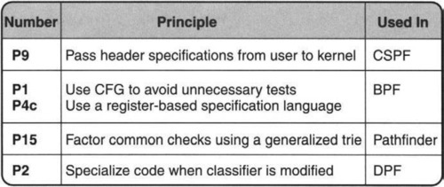
The demultiplexing techniques described in this chapter (and the corresponding principles used) are summarized in Figure 8.2.
8.1 OPPORTUNITIES AND CHALLENGES OF EARLY DEMULTIPLEXING
Why is early demultiplexing a good idea? The following basic motivations were discussed in Chapter 6.
• Flexible User-Level Implementations: The original reason for early demultiplexing was to allow flexible user-level implementation of protocols without excessive context switching.
• Efficient User-Level Implementations: As time went on, implementors realized that early demultiplexing could also allow efficient user-level implementations by minimizing the number of context switches. The main additional trick was to structure the protocol implementation as a shared library that can be linked to application programs.
However, there are other advantages of early demultiplexing.
• Prioritizing Packets: Early demultiplexing allows important packets to be prioritized and unnecessary ones to be discarded quickly. For example, Chapter 6 shows that the problem of receiver livelock can be mitigated by early demultiplexing of received packets to place packets directly on a per-socket queue. This allows the system to discard messages for slow processes during overload while allowing better behaved processes to continue receiving messages. More generally, early demultiplexing is crucial in providing quality- of-service guarantees for traffic streams via service differentiation. If all traffic is demultiplexed into a common kernel queue, then important packets can get lost when the shared buffer fills up in periods of overload. Routers today do packet classification for similar reasons (Chapters 12 and 14). Early demultiplexing allows explicit scheduling of the processing of data flows; scheduling and accounting can be combined to prevent anomalies such as priority inversion.
• Specializing Paths: Once the path for a packet is known, the code can be specialized to process the packet because the wider context is known. For example, rather than have each layer protocol check for packet lengths, this can be done just once in the spirit of P1, avoiding obvious waste. The philosophy of paths is taken to its logical conclusion in Mosberger and Peterson [MP96], who describe an operating system in which paths are first-class objects.
• Fast Dispatching: This chapter and Chapter 6 have already described an instance of this idea using packet filters and user-level protocol implementations. Early demultiplexing avoids per-layer multiplexing costs; more importantly, it avoids the control overhead that can sometimes be incurred in delayered multiplexing.
8.2 GOALS
If early demultiplexing is a good idea, is it easy to implement? Early demultiplexing is particularly easy to implement if each packet carries some information in the outermost (e.g., data link or network) header, which identifies the final endpoint. This is an example of P14, passing information in layer headers. For example, if the network protocol is a virtual circuit protocol such as ATM, the ATM virtual circuit identifier (VCI) can directly identify the final recipient of the packet.
However, protocols such as IP do not offer such a convenience. MPLS does offer this convenience, but MPLS is generally used only between routers, as described in Chapter 11. Even using a protocol such as ATM, the number of available VCIs may be limited. In lieu of a single demultiplexing field, more complex data structures are needed that we call packet filters or packet classifiers.
Such data structures take as input a complete packet header and map the input to an endpoint or path. Intuitively, the endpoint of a packet represents the receiving application process, while the path represents the sequence of protocols that need to be invoked in processing the packet prior to consumption by the endpoint. Before describing how packet filters are built, here are the goals of a good early-demultiplexing algorithm.
• Safety: Many early-demultiplexing algorithms are implemented in the kernel based on input from user-level programs. Each user program P specifies the packets it wishes to receive. As with Java programs, designers must ensure that incorrect or malicious users cannot affect other users.
• Speed: Since demultiplexing is done in real time, the early-demultiplexing code should run quickly, particularly in the case where there is only a single filter specified.
• Composability: If N user programs specify packet filters that describe the packets they expect to receive, the implementation should ideally compose these N individual packet filters into a single composite packet filter. The composite filter should have the property that it is faster to search through the composite filter than to search each of the N filters individually, especially for large N.
This chapter takes a mildly biological view, describing a series of packet filter species, with each successive adaptation achieving more of the goals than the previous one. Not surprisingly, the earliest species is nearly extinct, though it is noteworthy for its simplicity and historical interest.
8.3 CMU/STANFORD PACKET FILTER: PIONEERING PACKET FILTERS
The CMU/Stanford packet filter (CSPF) [MRA87] was developed to allow user-level protocol implementations in the Mach operating system. In the CSPF model, application programs provide the kernel with a program describing the packets they wish to receive. The program supplied by A operates on a packet header and returns true if the packet should be routed to application A. Like the old Texas Instrument calculators, the programming language is a stack-based implementation of an expression tree model.
As shown in Figure 8.3, the leaves of the tree represent simple test predicates on packet headers. An example of a test predicate is equality comparison with a fixed value; for example, in Figure 8.3, ETHER.TYPE = ARP represents a check of whether the Ethernet type field in the received packet matches the constant value specified for ARP (address resolution protocol) packets. The other nodes in the tree represent boolean operations such as AND and OR.
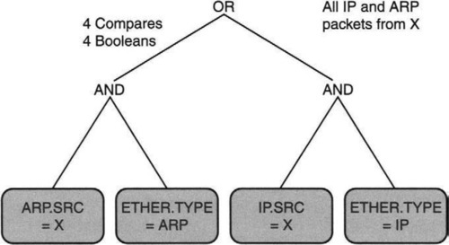
Thus the left subtree of the expression tree in Figure 8.3 represents any ARP packet sent from source IP address X, while the right subtree represents any IP packet sent from source IP address X. Since the root represents an OR operation, the overall tree asks for all IP or ARP packets sent by a source X. Such an expression could be provided by a debugging tool to the kernel on behalf of a user who wished to examine IP traffic coming from source X.
While the expression tree model provides a declarative model of a filter, such filters actually use an imperative stack-based language to describe expression trees. To provide safety, CSPF provides stack instructions of limited power; to bound running times there are no jumps or looping constructs. Safety is also achieved by checking program loads and stores in real time to eliminate wild memory references. Thus stack references are monitored to ensure compliance with the stack range, and references to packets are vetted to ensure they stay within the length of the packet being demultiplexed.
8.4 BERKELEY PACKET FILTER: ENABLING HIGH-PERFORMANCE MONITORING
CSPF guarantees security by using instructions of limited power and by doing run-time bounds checking on memory accesses. However, CSPF is not composable and has problems with speed. The next mutation in the design of packet filters occurred with the introduction of the Berkeley packet filter (BPF) [MJ93].
The BPF designers were particularly interested in using BPF as a basis for high-performance network-monitoring tools such as tcpdump, for which speed was crucial. They noted two speed problems with the use of even a single CSPF expression tree of the kind shown in Figure 8.3
• Architectural Mismatch: The CSPF stack model was invented for the PDP-11 and hence is a poor match to modern RISC architectures. First, the stack must be simulated at the price of an extra memory reference for each Boolean operation to update the stack pointer. Second, RISC architectures gain efficiency from storing variables in fast registers and doing computation directly from registers. Thus to gain efficiency in a RISC architecture, as many computations as possible should take place using a register value before it is reused. For instance, in Figure 8.3, the CSPF model will result in two separate loads from memory for each reference to the Ethernet type field (to check equality with ARP and IP). On modern machines, it would be better to reduce memory references by storing the type field in a register and finishing all comparisons with the type field in one fell swoop.
• Inefficient Model: Even ignoring the extra memory references required by CSPF, the expression tree model often results in more operations than are strictly required. For example, in Figure 8.3, notice that the CSPF expression takes four comparisons to evaluate all the leaves. However, notice that once we know that the Ethernet type is equal to ARP (if we are evaluating from left to right), then the extra check for whether the IP source address is equal to X is redundant (Principle P1, seek to avoid waste). The main problem is that in the expression tree model there is no way to “remember” packet parse state as the computation progresses. This can be fixed by a new model that builds a state machine.
CSPF had two other minor problems. It could only parse fields at fixed offsets within packet headers; thus it could not be used to access a TCP header encapsulated within an IP header, because this requires first parsing the IP header-length field. CSPF also processes headers using only 16-bit fields; this doubles the number of operations required for 32-bit fields such as IP addresses.
The Berkeley packet filter (BPF) fixes these problems as follows. First, it replaces the stack-based language with a register-based language, with an indirection operator that can help parse TCP headers. Fields at specified packet offsets are loaded into registers using a command such as “LOAD [12]”, which loads the Ethernet type field, which happens to start at an offset of 12 bytes from the start of an Ethernet packet.
BPF can then do comparisons and jumps such as “JUMP_IF_EQUAL ETHERTYPE_IP, TARGET1, TARGET2”. This instruction compares the accumulator register to the IP Ethernet type field; if the comparison is true, the program jumps to line number TARGET1; otherwise it jumps to TARGET2. BPF allows working in 8-, 16-, and 32-bit chunks.
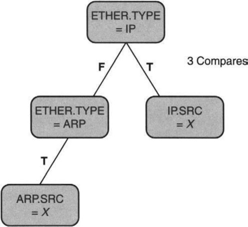
More fundamentally, BPF uses a control flow graph model of computation, as illustrated in Figure 8.4. This is basically a state machine starting with a root, whose state is updated at each node, following which it transitions to other node states, shown as arcs to other nodes. The state machine starts off by checking whether the Ethernet type field is that of IP; if true, it need only check whether the IP source field is X to return true. If false, it needs to check whether the Ethernet type field is ARP and whether the ARP source is X. Notice that in the left branch of the state machine we do not check whether the IP source address is X. Thus the worst-case number of comparisons is 3 in Figure 8.4, compared to 4 in Figure 8.3.
The Berkeley packet filter is used as a basis for a number of tools, including the well-known tcpdump tool by which users can obtain a readable transcript of TCP packets flowing on a link. BPF is embedded into the BSD kernel as shown in Figure 8.5.
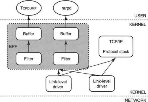
When a packet arrives on a network link, such as an Ethernet, the packet is processed by the appropriate link-level driver and is normally passed to the TCP/IP protocol stack for processing. However, if BPF is active, BPF is first called. BPF checks the packet against each currently specified user filter. For each matching filter, BPF copies as many bytes as are specified by the filter to a per-filter buffer. Notice that multiple BPF applications can cause multiple copies of the same packet to be buffered. The figure also shows another common BPF application besides tcpdump, the reverse ARP demon (rarpd).
There are two small features of BPF that are also important for high performance. First, BPF filters packets before buffering, which avoids unnecessary waste (P1) when most of the received packets are not wanted by BPF’s applications. The waste is not just memory for buffers but also for the time required to do a copy (Chapter 5).
Second, since packets can arrive very fast and the read() system call is quite slow, BPF allows batch processing (P2c) and allows multiple packets to be returned to the monitoring application in one call. To handle this and yet allow packet boundaries to be distinguished, BPF adds a header to each packet that includes a time stamp and length. Users of tcpdump do not have to use this interface; instead, tcpdump offers a more user-friendly interface: Interface commands are compiled to BPF instructions.
8.5 PATHFINDER: FACTORING OUT COMMON CHECKS
BPF is a more refined adaptation than CSPF becauses it increases speed for a single filter. However, every packet must still be compared with each filter in turn. Thus the processing time grows with the number of filters. Fortunately, this is not a problem for typical BPF usage. For example, a typical Tcpdump application may provide only a few filters to BPF.
However, this is not true if early demultiplexing is used to discriminate between a large number of packet streams or paths. In particular, each TCP connection may provide a filter, and the number of concurrent TCP connections in a busy server can be large. The need to deal with this change in environment (user-level networking) led to another successful mutation, called Pathfinder [BGP+94], Pathfinder goes beyond BPF by providing composability. This allows scaling to a large number of users.
To motivate the Pathfinder solution, imagine there are 500 filters, each of which is exactly the same (Ethernet type field is IP, IP protocol type is TCP) except that each specifies a different TCP port pair. Doing each filter sequentially would require comparing the Ethernet type of the packet 500 times against the (same) IP Ethernet type field and comparing the IP protocol field 500 times against the (same) TCP protocol value. This is wasteful (P1).
Next, comparing the TCP port numbers in the packet to each of the 500 port pairs specified in each of the 500 filters is not obvious waste. However, this is exactly analogous to a linear search for exact matching. This suggests that integrating all the individual filters into a single composite filter can considerably reduce unnecessary comparisons when the number of individual filters is large. Specifically, this can be done using hashing (P15, using efficient data structures) to perform exact search; this can replace 500 comparisons with just a few comparisons.
A data structure for this purpose is shown in Figure 8.6. The basic idea is to superimpose the CFGs for each filter in BPF so that all comparisons on the same field are placed in a single node. Finally, each node is implemented as a hash table containing all comparison values to replace linear search with hashing.
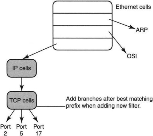
Figure 8.6 shows an example with at least four filters, two of which specify TCP packets with destination port numbers 2 and 5; for now ignore the dashed line to TCP port 17, which will be used as an example of filter insertion in a moment. Besides the TCP filters, there are one or more filters that specify ARP packets and one or more filters that specify packets that use the OSI protocol.
The root node corresponds to the Ethernet type field; the hash table contains values for each possible Ethernet type field value used in the filters. Each node entry has a value and a pointer. Thus the ARP entry points to nodes that further specify what type of ARP packets must be received; the OSI entry does likewise. Finally, the Ethernet type field corresponding to IP points to a node corresponding to the IP protocol field.
In the IP protocol field node, one of the values corresponding to TCP (which has value 6) will point to the TCP node. In the TCP node, there are three values pointing to the three possible destination port values of 2 and 5 (recall that the 17 has not been inserted yet). When a TCP packet arrives, demultiplexing proceeds as follows.
Search starts at the root, and the Ethernet type field is hashed to find a matching value corresponding to IP. The pointer of this value leads to the IP node, where the IP protocol type field is hashed to find a matching value corresponding to TCP. The value pointer leads to the TCP node, where the destination port value in the packet is hashed to lead to the final matching filter.
The Pathfinder data structure has a strong family resemblance to a common data structure called a trie, which is more fully described in Chapter 11. Briefly, a trie is a tree in which each node contains an array of pointers to subtries; each array contains one pointer for each possible value of a fixed-character alphabet.
To search the trie for a keyword, the keyword is broken into characters, and the ith character is used to index into the ith node on the path, starting with the root. Searching in this way at node i yields a pointer that leads to node i + 1, where search continues recursively. One can think of the Pathfinder structure as generalizing a trie by using packet header fields (e.g., Ethernet type field) as the successive characters used for search and by using hash tables to replace the arrays at each node.
It is well known that tries provide fast insertions of new keys. Given this analogy, it is hardly surprising that Pathfinder has a fast algorithm to insert or delete a filter. For instance, consider inserting a new filter corresponding to TCP port 17. As in a trie, the insert algorithm starts with a search for the longest matching prefix (Chapter 11) of this new filter.
This longest match corresponds to the path Ethernet Type = IP and IP Protocol = TCP. Since this path has already been created by the other two TCP filters, it need not be replicated. The insertion algorithm only has to add branches (in this case, a single branch) corresponding to the portion of the new filter beyond the longest match. Thus the hash table in the TCP node need only be updated to add a new pointer to the port 17 filter.
More precisely, the basic atomic unit in Pathfinder is called a cell. A cell specifies a field of bits in a packet header (using an offset, length, and a mask), a comparison value, and a pointer. For example, ignoring the pointer, the cell that checks whether the IP protocol field is TCP is (9, 1, 0xff, 6) — the cell specifies that the ninth byte of the IP header should be masked with all l’s and compared to the value 6, which specifies TCP.
Cells of a given user are strung together to form a pattern for that user. Multiple patterns are superimposed to form the Pathfinder trie by not recreating cells that already exist. Finally, multiple cells that specify identical bit fields but different values are coalesced using a hash table.
Besides using hash tables in place of arrays, Pathfinder also goes beyond tries by making each node contain arbitrary code. In effect, Pathfinder recognizes that a trie is a specialized state machine that can be generalized by performing arbitrary operations at each node in the trie. For instance, Pathfinder can handle fragmented packets by allowing loadable cells in addition to the comparison cells described earlier. This is required because for a fragmented packet only the first fragment specifies the TCP headers; what links the fragments together is a common packet ID described in the first fragment.
Pathfinder handles fragmentation by placing an additional loadable cell (together with the normal IP comparison cell specifying, say, a source address) that is loaded with the packet ID after the first fragment arrives. A cell is specified as loadable by not specifying the comparison value in a cell.
The loadable cell is not initially part of the Pathfinder trie but is instead an attribute of the IP cells. If the first fragment matches, the loaded cell is inserted into the Pathfinder trie and now matches subsequent fragments based on the newly loaded packet ID. After all fragments have been removed, this newly added cell can be removed. Finally, Pathfinder handles the case when the later fragments arrive before the first fragment by postponing their processing until the first fragment arrives.
Although Pathfinder has been described so far as a tree, the data structure can be generalized to a directed acyclic graph (DAG). A DAG allows two different filters to initially follow different paths through the Pathfinder graph and yet come together to share a common path suffix. This can be useful, for instance, when providing a filter for TCP packets for destination port 80 that can be fragmented or unfragmented. While one needs a separate path of cells to specify fragmented and unfragmented IP packets, the two paths can point to a common set of TCP cells.
Finally, Pathfinder also allows the use of OR links that lead from a cell. The idea is that each of the OR links specify a value, and each of the OR links is checked to find a value that matches and then that link is followed.
In order to prioritize packets during periods of congestion, as in Chapter 6, the demultiplexing routine must complete in the minimum time it takes to receive a packet. Software implementations of Pathfinder are fast but are typically unable to keep up with line speeds. Fortunately, the Pathfinder state machine can be implemented in hardware to run at line speeds. This is analogous to the way IP lookups using tries can be made to work at line speeds (Chapter 11).
The hardware prototype described in Bailey et al. [BGP+94] trades functionality for speed. It works in 16-bit chunks and implements only the most basic cell functions; it does, however, implement fragmentation in hardware. The limited functionality implies that the Pathfinder hardware can only be used as a cache to speed up Pathfinder software that handles the less common cases. A prototype design running at 100 MHz was projected to take 200 nsec to process a 40-byte TCP message, which is sufficient for 1.5 Gbps. The design can be scaled to higher wire speeds using faster clock rates, faster memories, and a pipelined traversal of the state machine.
8.6 DYNAMIC PACKET FILTER: COMPILERS TO THE RESCUE
The Pathfinder story ends with an appeal to hardware to handle demultiplexing at high speeds. Since it is unlikely that most workstations and PCs today can afford dedicated demultiplexing hardware, it appears that implementors must choose between the flexibility afforded by early demultiplexing and the limited performance of a software classifier. Thus it is hardly surprising that high-performance TCP [CJRS89], active messages [vCGS92], and Remote Procedure Call (RPC) [TNML93] implementations use hand-crafted demultiplexing routines.
Dynamic packet filter [EK96] (DPF) attempts to have its cake (gain flexibility) and eat it (obtain performance) at the same time. DPF starts with the Pathfinder trie idea. However, it goes on to eliminate indirections and extra checks inherent in cell processing by recompiling the classifier into machine code each time a filter is added or deleted. In effect, DPF produces separate, optimized code for each cell in the trie, as opposed to generic, unoptimized code that can parse any cell in the trie.
DPF is based on dynamic code generation technology [Eng96], which allows code to be generated at run time instead of when the kernel is compiled. DPF is an application of Principle P2, shifting computation in time. Note that by run time we mean classifier update time and not packet processing time.
This is fortunate because this implies that DPF must be able to recompile code fast enough so as not to slow down a classifier update. For example, it may take milliseconds to set up a connection, which in turn requires adding a filter to identify the endpoint in the same time. By contrast, it can take a few microseconds to receive a minimum-size packet at gigabit rates. Despite this leeway, submillisecond compile times are still challenging.
To understand why using specialized code per cell is useful, it helps to understand two generic causes of cell-processing inefficiency in Pathfinder:
• Interpretation Overhead: Pathfinder code is indeed compiled into machine instructions when kernel code is compiled. However, the code does, in some sense, “interpret” a generic Pathfinder cell. To see this, consider a generic Pathfinder cell C that specifies a 4-tuple: offset, length, mask, value. When a packet P arrives, idealized machine code to check whether the cell matches the packet is as follows:
LOAD R1, C(Offset); (* load offset specified in cell into register R1 *)
LOAD R2, C(length); (* load length specified in cell into register R1 *)
LOAD R3, P(R1, R2); (* load packet field specified by offset into R3 *)
LOAD R1, C(mask); (* load mask specified in cell into register R1 *)
AND R3, R1; (* mask packet field as specified in cell *)
LOAD R2, C(value); (* load value specified in cell into register R5 *)
BNE R2, R3; (* branch if masked packet field is not equal to value *)
Notice the extra instructions and extra memory references in Lines 1, 2, 4, and 6 that are used to load parameters from a generic cell in order to be available for later comparison.
• Safety-Checking Overhead: Because packet filters written by users cannot be trusted, all implementations must perform checks to guard against errors. For example, every reference to a packet field must be checked at run time to ensure that it stays within the current packet being demultiplexed. Similarly, references need to be checked in real time for memory alignment; on many machines, a memory reference that is not aligned to a multiple of a word size can cause a trap. After these additional checks, the code fragment shown earlier is more complicated and contains even more instructions.
By specializing code for each cell, DPF can eliminate these two sources of overhead by exploiting information known when the cell is added to the Pathfinder graph.
• Exterminating Interpretation Overhead: Since DPF knows all the cell parameters when the cell is created, DPF can generate code in which the cell parameters are directly encoded into the machine code as immediate operands. For example, the earlier code fragment to parse a generic Pathfinder cell collapses to the more compact cell-specific code:
LOAD R3, P(offset, length); (* load packet field into R3 *)
AND R3, mask; (* mask packet field using mask in instruction *)
BNE R3, value; (* branch if field not equal to value *)
Notice that the extra instructions and (more importantly) extra memory references to load parameters have disappeared, because the parameters are directly placed as immediate operands within the instructions.
• Mitigating Safety-Checking Overhead: Alignment checking can be reduced in the expected case (P11) by inferring at compile time that most references are word aligned. This can be done by examining the complete filter. If the initial reference is word aligned and the current reference (offset plus length of all previous headers) is a multiple of the word length, then the reference is word aligned. Real-time alignment checks need only be used when the compile time inference fails, for example, when indirect loads are performed (e.g., a variable-size IP header). Similarly, at compile time the largest offset used in any cell can be determined and a single check can be placed (before packet processing) to ensure that the largest offset is within the length of the current packet.
Once one is onto a good thing, it pays to push it for all it is worth. DPF goes on to exploit compile-time knowledge in DPF to perform further optimizations as follows. A first optimization is to combine small accesses to adjacent fields into a single large access. Other optimizations are explored in the exercises.
DPF has the following potential disadvantages that are made manageable through careful design.
• Recompilation Time: Recall that when a filter is added to the Pathfinder trie (Figure 8.6), only cells that were not present in the original trie need to be created. DPF optimizes this expected case (P11) by caching the code for existing cells and copying this code directly (without recreating them from scratch) to the new classifier code block. New code must be emitted only for the newly created cells. Similarly, when a new value is added to a hash table (e.g., the new TCP port added in Figure 8.6), unless the hash function changes, the code is reused and only the hash table is updated.
• Code Bloat: One of the standard advantages of interpretation is more compact code. Generating specialized code per cell appears to create excessive amounts of code, especially for large numbers of filters. A large code footprint can, in turn, result in degraded instruction cache performance. However, a careful examination shows that the number of distinct code blocks generated by DPF is only proportional to the number of distinct header fields examined by all filters. This should scale much better than the number of filters. Consider, for example, 10,000 simultaneous TCP connections, for which DPF may emit only three specialized code blocks: one for the Ethernet header, one for the IP header, and one hash table for the TCP header.
The final performance numbers for DPF are impressive. DPF demultiplexes messages 13–26 times faster than Pathfinder on a comparable platform [EK96]. The time to add a filter, however, is only three times slower than Pathfinder. Dynamic code generation accounts for only 40% of this increased insertion overhead.
In any case, the larger insertion costs appear to be a reasonable way to pay for faster demultiplexing. Finally, DPF demultiplexing routines appear to rival or beat hand-crafted demultiplexing routines; for instance, a DPF routine to demultiplex IP packets takes 18 instructions, compared to an earlier value, reported in Clark [Cla85], of 57 instructions. While the two implementations were on different machines, the numbers provide some indication of DPF quality.
The final message of DPF is twofold. First, DPF indicates that one can obtain both performance and flexibility. Just as compiler-generated code is often faster than hand-crafted code, DPF code appears to make hand-crafted demultiplexing no longer necessary. Second, DPF indicates that hardware support for demultiplexing at line rates may not be necessary. In fact, it may be difficult to allow dynamic code generation on filter creation in a hardware implementation. Software demultiplexing allows cheaper workstations; it also allows demultiplexing code to benefit from processor speed improvements.
8.7 CONCLUSIONS
While it may be trite to say that necessity is the mother of invention, it is also often true. New needs drive new innovations; the lack of a need explains why innovations did not occur earlier. The CSPF filter was implemented when the major need was to avoid a process context switch; having achieved that, improved filter performance was only a second-order effect. BPF was implemented when the major need was to implement a few filters very efficiently to enable monitoring tools like tcpdump to run at close to wire speeds. Having achieved that, scaling to a large number of filters seemed less important.
Pathfinder was implemented to support user-level networking in the x-kemel [HP91], and to allow Scout [MP96] to use paths as a first-class object that could be exploited in many ways. Having found a plausible hardware implementation, perhaps improved software performance seemed less important. DPF was implemented to provide high-performance networking together with complete application-level flexibility in the context of an extensible operating system [EKO95]. Figure 8.2 presents a summary of the techniques used in this chapter, together with the major principles involved.
As in the H. G. Wells quote at the start of the chapter, the DPF species does represent the accumulation of the experiments of all its successful individuals. All filter implementations borrow from CSPF the intellectual leap of separating demultiplexing from packet processing, together with the notion that application demultiplexing specifications can be safely exported to the kernel. DPF and Pathfinder in turn borrow from BPF the basic notion of exploiting the underlying architecture using a register-based, state-machine model. DPF borrows from Pathfinder the notion of using a generalized trie to factor out common checks.
8.8 EXERCISES
1. Other Uses of Early Demultiplexing: Besides the uses of early demultiplexing already described, consider the following potential uses.
• Quality of Service: Why might early demultiplexing help offer different qualities of service to different packets in an end system? Give an example.
• Integrated Layer Processing: Integrated layer processing (ILP) was studied in Chapter 5. Discuss why early demultiplexing may be needed for ILP.
• Specializing Code: Once the path of a protocol is known, one can possibly specialize the code for the path, just as DPF specializes the code for each node. Give an example of how path information could be exploited to create more efficient code.
2. Further DPF Optimizations: Besides the optimizations already described consider the following other optimizations that DPF exploits.
• Atom Coalescing: It often happens that a node in the DPF tree checks for two smaller field values in the same word. For example, the TCP node may check for a source port value and a destination port value. How can DPF do these checks more efficiently? What crucial assumption does this depend on, and how can DPF validate this assumption?
• Optimizing Hash Tables: When DPF adds a classifier, it may update the hash table at the node. Unlike Pathfinder, the code can be specialized to the specific set of values in each hash table. Explain why this can be used to provide a more efficient implementation for small tables and for collision handling in some cases.