Unicode, UTF, and ASCII

As noted previously, Unicode isn’t an encoding scheme, it is a standard for relating code points to characters. The Unicode standard specifies up to 1,114,112 code points, each of which is stored in one of 16 65,536-point code planes. We care primarily about plane zero, which contains all the characters in the sets listed in Table 12-1.

Encoding, which is to say the process of actually representing the characters, is managed primarily via UTF-8 (Unicode Text Format, RFC 3629). UTF-8 is a variable-length encoding scheme specifically designed to handle a number of problems involved in transmission and in its predecessor standard, UTF-16. This means that Unicode encoding has a number of header and delimiter conventions that limit the efficiency of the system. The value 129, for instance, is going to stretch across 2 bytes. The following example shows this in action, as well as the germane Python commands:

# This is done in Python 2.7; the Python 3 version merges the uni*
# functions for ease of use.
>>> s=unichr(4E09)
# unichr is the Unicode equivalent of chr; note that I enter the
# hexadecimal index.  All it cares about is the index value.
>>> print(s)
三
>>> print(unichr(19977))
三
# print is important, direct text dump is going to give me the
# abstract Unicode encoding that Python uses.  Note the u and u
# characters.  The u before the string indicates it's Unicode,
# the u indicates it's an unsigned sixteen bit--Python effectively
# uses UTF-16 internally for representation.
>>> s
u'u4e09'
# Now, let's convert from utf-16 to utf-8.
>>> s.encode('utf-8')
'xe4xb8x89'
# Note that this is 3 bytes; a utf-8 representation includes
# overhead to describe the data provided.  Let's compare it
# with vanilla ASCII.
>>> s=u'a'
>>> print s
a
>>> s
a
# Note that we're in ASCIIland and it's treated as a default.
>>> s.encode('utf-8')
'a'
>>> ord(s)
97

Note that in the example, as soon as I went to the a character, the encoding function and everything else dropped all of the hexadecimal and integer encoding. UTF-8 is backward compatible with ASCII (American Standard Code for Information Interchange), the 7-bit⁶ character encoding standard.

Encoding for Attackers

Having discussed the general role of encoding, now let’s talk about the role of encoding for an attacker. For attackers, encoding is a tool for evasion, slipping information past filters intended to stop them, delaying defenders from figuring out that something is amiss. To that end, the attackers can rely on a number of different techniques to manipulate encoding, abetted by the implicit dependencies encoding strategies have.

Base64 encoding

Base encoding⁷ is an encoding technique originally developed for email that currently serves as a workhorse for data transfer, including malware.

The goal of base64 encoding is to provide a mechanism for encoding arbitrary binary values using commonly recognized characters. To do so, it maps binary values to values between 0 and 63, assigns each code point a common, easily recognizable character, and then encodes the values using that character. The base64 encoding standard involves 64 code points representing the characters A–Z, a–z, and 0–9, and two characters that differ by standard—we’ll say + and / for now.

Figure 12-1 shows the basic process of base64 encoding. Note that the process includes a padding convention; when working with bytes, base64 encoding neatly transfers 3 bytes into 4 characters. If your string isn’t a multiple of three, you’ll need to zero-pad up to three and then add equals signs at the end of the encoded string to indicate this.

Figure 12-1. Base64 encoding in action

Base64 encoding is cheap and omnipresent; Python includes a standard library in the form of base64, and JavaScript has btoa and atob functions to handle it. This makes it a pretty easy and quick way to hide text directly.

In addition to base64, HTML natively supports a completely different encoding, called numeric character references (NCRs). Numeric character references encode values using the format &#DDDD;, where DDDD is the index of the corresponding code point in Unicode. NCRs can use decimal (e.g., 三) or hex (e.g., &#0x4E09;).

The fastest way to identify base64 is to look for characters that base64 doesn’t cover, but which you expect to see: commas, spaces, periods, and apostrophes. Long sequences of text without those will be unusual. NCRs are recognizable by the use of ampersands.

Finding a String

The go-to tool for finding a particular string is grep (the generalized regular expression processor). When using grep, remember that its default input is regular expressions—consequently, when entering IP addresses, you can run into overmatches. For example:

$ grep 10.16 http_example.txt  | grep '10:16'
10.147.201.99 - - [17/Sep/2016:10:16:14 -0400] "HEAD / HTTP/1.1" 200 221 "-" "-"
10.147.201.99 - - [17/Sep/2016:10:16:16 -0400] "GET / HTTP/1.1" 200 2357 "-" "-"
$ grep 10.16 http_example.txt  | grep -v '10:16' | head -1
10.16.94.206 - - [18/Sep/2016:05:57:16 -0400] "GET
   /helpnew/faq/faq_simple_zh_CN.jsp HTTP/1.1" 404 437 "-"
   "Mozilla/5.0 (Macintosh; Intel Mac OS X 10_9_4) AppleWebKit/537.36
   (KHTML, like Gecko) Chrome/36.0.1985.125 Safari/537.36"

Since the . character is a wildcard in regular expressions, grep looks for both the address and the time signature. Ensure that you match a literal dot using the . construct:

$ grep '10.16' http_example.txt | head -1
10.16.94.206 - - [18/Sep/2016:05:57:16 -0400] 
  "GET /helpnew/faq/faq_simple_zh_CN.jsp HTTP/1.1" 404 437 "-" 
  "Mozilla/5.0 (Macintosh; Intel Mac OS X 10_9_4) AppleWebKit/537.36 
    (KHTML, like Gecko) Chrome/36.0.1985.125 Safari/537.36"

Python strings support two searching methods: find and index. Of the two, I prefer find over index purely because index raises an exception when it fails to find a string. I’m intentionally avoiding discussing the re library for now; I’ll discuss regular expressions a bit more later.

Manipulating Delimiters

The tr tool provides a number of handy utilities for splitting delimiters. Without other switches, tr will do an ordered substitution of the contents of one list with another list. Here’s an example of how this works:

$ echo 'dog cat god' | tr 'dog' 'bat'
bat cat tab

As the example shows, tr transposes the individual characters, not the entire string. To do this in Python, you need to use a string’s .translate method. This method takes a translation table, which is best generated using the maketrans function from the string library. Here’s an example:

>>> from string import maketrans
>>> 'dog cat god'.translate(maketrans('dog','bat'))
'bat cat tab'

tr includes a number of other handy routines, the most important one being -s. The squeeze operation will reduce multiple copies of a specified character down to one, particularly important when working with spaces. For example:

$ echo 'a||b|c' | tr -s '|'
a|b|c

The most Pythonic way to do this is to split the series into a list, filter out empty elements, and then join the list using the original delimiter. For example:

>>> '|'.join(filter(bool, 'a||b|c'.split('|')))
'a|b|c'

Splitting Along Delimiters

cut is capable of splitting files along delimiters, characters, bytes, or other values as needed. To use delimiters, specify a -d argument and then a -f for the fields:

$ echo 'a|b|c' | cut -d '|' -f 3,1
a|c

Note that -f doesn’t pay attention to the ordering—you get the fields in the order they appear in the file. Also note that the -d argument takes a single character.

In Python, the .split method converts strings to lists, after which you can manipulate them as normal. Given how Python slicing works, it’s generally preferable to use the itemgetter function after that to get ordered elements:

>>> from operator import itemgetter
>>> itemgetter(2,1,5)('a|b|c|d|e|f'.split('|'))
('c', 'b', 'f')

In passing, NumPy arrays provide an arbitrary selection operator via double brackets ([[).

Regular Expressions

Regular expressions are the most powerful tool directly available for text analysis. In this section, I will provide a very brief overview of their use, as well as some rules for ensuring that they don’t get out of hand. In general, my largest caution about using regular expressions is that they are very expensive—regular expressions are effectively an interpreted programming language for matching text, and there are often much more effective and faster mechanisms for achieving the same results, such as tr.

A regular expression is a sequence of characters specifying how to match another sequence of characters. In its simplest form, a regular expression is just a string. Here is an example of regular expression matching in Python:

>>> import re
>>> re.search('foo','foobar')
<_sre.SRE_Match object at 0x100431cc8>
>>> re.search('foo','waffles')

Python regular expressions are implemented by the re library. As this example shows, a successful regular expression search will return a match object; a failure of the search function will return None.

The re library contains three key functions: search, match, and findall. search searches through the target string and terminates on the first match; match succeeds only on an exact match. Both search and match return match objects on success, or None on failure. findall will search for every instance of a regular expression and return a list of successful matches:

>>> re.match('foo','foobar')
<_sre.SRE_Match object at 0x100431cc8>
>>> re.match('foo','barfoo')
# Note the failure; this is because of the positioning of foo - the characters
# bar precede it.
>>> re.search('foo','foobar')
<_sre.SRE_Match object at 0x1004318b8>
>>> re.search('foo','barfoo')
<_sre.SRE_Match object at 0x100431cc8>
# Search works because it isn't an exact match
>>> re.findall('foo','foofoo')
['foo', 'foo']

Regular expressions provide a rich language for wildcarding. The most basic wildcards involve the use of the ., ?, +, and * characters. . specifies a match for a single character, while the other three specify the order of the match. ? indicates zero or one instances, + one or more, and * zero or more:

>>> re.findall('foo.+','foo foon foobar')
['foo foon foobar']
>>> re.findall('foo.?','foo foon foobar')
['foo ', 'foon', 'foob']
>>> re.findall('foo.','foo foon foobar')
['foo foon foobar']
>>> re.findall('foo*','foo foon foobar')
['foo', 'foo', 'foo']
>>> re.findall('foo.*','foo foon foobar')
['foo ', 'foon', 'foob']

Instead of simply matching on one or more characters, regular expressions can be grouped into parentheses. The order characters can then be applied to the whole expression:

>>> re.findall('f(o)+','foo foooooo')
['o', 'o']
>>> re.findall('f(o)+','foo')
['o']

When you use a group, the matches will only return the characters in the group. This is handy for extracting specific terms. For example:

>>> re.findall('To: (.+)','To: Bob Smith <[email protected]>')
['Bob Smith <[email protected]>']
>>> re.findall('To: (.+) <','To: Bob Smith <[email protected]>')
['Bob Smith']
>>> re.findall('To: (.+) <(.*)>','To: Bob Smith <[email protected]>')
[('Bob Smith', '[email protected]')]

Groups can also express a number of options, via a bar, and a specific number of instances by putting the range in curly braces:

>>> re.findall('T(a|b)','To Ta Tb To Tb Ta')
['a', 'b', 'b', 'a']
>>> re.findall('T(a){2,4}','To Ta Taa Taaa')
['a', 'a']

Square brackets are used to match a range of characters:

>>> re.findall('f[abc]','fo fa fb fo fc')
['fa', 'fb', 'fc']

Finally, a couple of special notes. The ^ and $ symbols are used to match the beginning and end of a string:

>>> re.findall('^f[o]+','foo fooo')
['foo']
>>> re.findall('f[o]+','foo fooo')
['foo', 'fooo']
>>> re.findall('f[o]+$','foo fooo fo')
['fo']

You can match any of the control characters (e.g., {, +, etc.) by slapping a in front of them:

>>> re.findall('a+.','ab a+b')
['a+b']

That was a very basic introduction to regular expressions, but I’ll also make some practical observations.

First, if you’re using regular expression matching with a new tool, check to see how much regular expression parsing the tool does. At the minimum, regular expressions tend to be broken into a basic syntax, an extended syntax (ERE), and PCRE (Perl Compatible Regular Expression) syntax. The default grep tool, for example, doesn’t recognize extended syntax, so the first command here produces no output:

$ echo 'foo' | grep 'fo.?'
$ echo 'foo' | egrep 'fo.?'
foo

Most modern environments will use ERE, and everything I’ve discussed in this chapter should work if the parser recognizes ERE. PCRE, yet more powerful, usually requires additional libraries, and there is a standard PCRE tool (pcregrep) for parsing those expressions. If you expect to be doing a lot of Unicode work, I suggest going straight to PCRE.

Second, keep notes. Outside of one-off parsing, you’re most likely going to use regular expressions to repeatedly parse and normalize logfiles as part of the analysis infrastructure. The logfile format changes, regular expressions fail, and you’re left trying to figure out what that string of line noise actually means. A useful aid to this documentation process is to use capture groups, to ensure that you can track what you’re watching for.

Third, use regular expressions for what they’re good for, and keep them simple. Matching string. is an expensive way to match string. As a rule of thumb, if I’m not doing something at least as complex as a conditional (e.g., (a|b)) or a sequence count (e.g., a{2,3}), I’m looking for a simpler approach. Regular expressions are expensive—many common tasks, such as squeezing spaces, are three to four times slower using REs.

Finally, if you’re working in Python, make sure you’re compiling, and know the difference between match and search and findall. Since match requires that you express the full string, it tends to necessitate a considerable amount more complexity and performance than search does.

N-Gram Analysis

An n-gram is a sequence of n or more tokens. For example, when parsing characters in a text string, an n-gram will be n or more individual characters in sequence, such as turning “waffles” into the trigrams “waf”, “aff”, “ffl”, “fle”, and “les”. The same principle can be used for words in a sentence (“I have”, “have pwnd”, “pwnd your”, “your system”) or any other token.

The key feature of n-gram decomposition is the use of this sliding window. n-gram decompositions produce a lot of strings from a single source, and the process of analyzing the n-grams is computationally expensive. However, n-gram analysis is, in my experience, a very good “I don’t know what’s in this data yet” technique when you’re looking at previously unknown piles of text. With many of the following distance techniques, you may use them interchangeably with the original strings or with n-grams.

Jaccard Distance

Of the three comparison metrics I will discuss in this section, the Jaccard distance is the cheapest to implement, but also the least powerful. Given two strings, A and B, the Jaccard distance is calculated as the ratio of the intersection of A and B over the union of A and B. Jaccard distance is trivial to calculate using Python’s set operators, as shown here:

def jaccard(a,b):
    """
    Given two strings a and b, calculate the Jaccard distance
    between them as characters
    """
    set_a = set(a)
    set_b = set(b)
    return float(len((set_a.intersection(set_b))))/float(len(set_a.union(set_b)))

Jaccard distance is quick to implement, and it’s easy to implement a very fast version of the set when you know all the potential tokens. It’s also normalized: a value of 0 indicates no characters in common, and 1 indicates that all characters are in common. That said, it’s not a very powerful distance metric—it doesn’t account for duplicated characters, string ordering, or the presence of substrings, so the strings “foo” and “ofoffffoooo” are considered as identical as “foo” and “foo”.

Hamming Distance

The Hamming distance between two strings of identical length is the total number of individual characters within those strings that differ. This is shown in Python in the following example:

def hamming(a,b):
    """
    Given two strings of identical length, calculate the Hamming
    distance between them.
    """
    if len(a) == len(b):
	return sum(map(lambda x:1 if x[0] == x[1] else 0, zip(a,b)))
    else:
	raise Exception, "Strings of different length"

Hamming distance is a powerful similarity metric. It’s fast to calculate, but it’s also restricted by string size, and the lack of normalization means that the values are a little vague. In addition, when you calculate a Hamming distance, you have to be very clear about what your definition of a different token is. For example, if you decide to use individual bits as a distance metric, you will find that UTF-16 encodings and UTF-8 encodings of the same strings will have different values due to the encoding overheads!

Levenshtein Distance

The Levenshtein distance between two strings is described as the minimum number of single character operations (insertions, deletions, or character substitutions) required to change one string to another string. For example, the strings “hax0r” and “hacker” have a Levenshtein distance of 3 (add a c before the x, change x to k, change 0 to e).

Levenshtein distance is one of those classic “let’s learn dynamic programming” examples, and is a bit more complex than I want to dive into in this chapter. The leven​shtein function in text_examples.py provides an example of how to implement this distance metric.

Levenshtein distance is sensitive to substrings and placement in ways that Hamming distance isn’t. For example, the strings “hacks” and “shack” have a Hamming distance of 5 but a Levenshtein distance of 2 (add an s at the beginning, drop an s from the end). However, it’s a considerably more computationally expensive algorithm to implement than Hamming distance, and you may end up paying a performance cost for identifying phenomena that are discernible using a cheaper algorithm.

Entropy and Compressibility

The entropy (properly, Shannon entropy) of a signal is the probability that a particular character will appear in a sample of that signal. This is mathematically formulated as:

That is, the sum over all the observed symbols of their probabilities by their information content (the log of their entropy).

The entropy as formulated here describes the number of bits required to describe all of the characters observed in a string. So, the entropy of the string “abcd” would be 2 (there are four unique symbols), and the entropy of the string “abcedfgh” would be 3 (8 unique symbols). Signals that are high-entropy are noisy—they look like the data is randomly generated, as the probability of seeing any particular token is largely even. Low-entropy signals are biased toward repeated patterns; as a rule of thumb, low-entropy data is structured, has repeated symbols, and is compressible.

Natural language is low-entropy, and most logfiles are low-entropy; compressed data is high-entropy (compression is about finding entropy and exploiting it), and encrypted data is high-entropy (because the goal is to look like noise). Figure 12-3 shows this phenomenon in more depth; this figure shows the results, respectively, of compressing and encrypting data (in this case, 10,000-character samples of the complete works of Shakespeare). As the example illustrates, the entropy of natural-language text hovers at around 5 bits/character, while that of compressed and encrypted data is approximately 8 bits/character.

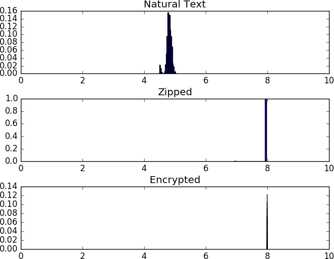
Figure 12-3. A comparison of entropy for different systems

Selectively sampling and approximating entropy is a good quick-and-dirty technique to check for compression or encryption on a dataset.

Homoglyphs

In http_example.txt, there’s a line that reads:

10.193.9.88 - - [19/Sep/2016:19:36:11 -0400] "POST
/wp-loаder.php HTTP/1.1" 404 380 "-" "Mozilla/5.0
(Windows NT 6.0; rv:16.0) Gecko/20130722 Firefox/16.0"

Let’s look for it:

$ cat http_example.txt | grep loader
$ cat http_example.txt | grep 10.193.9.88
10.193.9.88 - - [19/Sep/2016:19:36:11 -0400] "POST
/wp-loаder.php HTTP/1.1" 404 380 "-" "Mozilla/5.0
(Windows NT 6.0; rv:16.0) Gecko/20130722 Firefox/16.0"

What sorcery is this? The a in the logfile is actually the Unicode character 0x430, or the Cyrillic lowercase a. Thus, the first request returns no results. This is an example of a homoglyph—two code points with identical-appearing glyphs. Homoglyph attacks rely on this similarity; to the human eye the characters look identical, but they are encoded differently and an analyst grepping for the former will not find the latter.

Homoglyphs are a particular problem when dealing with the DNS. Internationalized domain names (IDNs) include mechanisms to ease the process of creating multi-code-page domain names, resulting in demonstrated attacks. Unfortunately, there’s no fast and easy way to determine whether something is a homoglyph—they are literally fooling sight. Generally, the best rule of thumb is to try to work within a specific code page (such as in the US, catching anything with a character code above 127). Alternatively, there are tables of known homoglyphs (see the next section for more information) that can provide you with lists of characters to watch out for.