
![]()
The End of Disk? SSD and In-Memory Databases
640K of memory should be enough for anybody.
—attributed (without foundation) to Bill Gates, 1981
I’ve said some stupid things and some wrong things, but not that.
—Bill Gates, 2001
Ever since the birth of the first database systems, database professionals have strived to avoid disk IO at all costs. IO to magnetic disk devices has always been many orders of magnitude slower than memory or CPU access, and the situation has only grown worse as Moore’s law accelerated the performance of CPU and memory while leaving mechanical disk performance behind.
The emergence of affordable solid state disk (SSD) technology has allowed for a quantum leap in database disk performance. Over the past few years, SSD technology has shifted from an expensive luxury to a mainstream technology that has a place in almost every performance-critical database system. However, SSDs have some unique performance characteristics and some database systems have been developed to exploit these capabilities.
While SSDs allow IO to be accelerated, the increasing capacity and economy of server memory sometimes allows us to avoid IO altogether. Many smaller databases can now fit entirely within the memory capacity of a single server, and certainly within the memory capacity of a cluster. For these databases, an in-memory solution may be even more attractive than an SSD architecture.
The End of Disk?
The magnetic disk device has been a pervasive presence within digital computing since the 1950s. The essential architecture has changed very little over that time: one or more platters contain magnetic charges that represent bits of information. These magnetic charges are read and written by an actuator arm, which moves across the disk to a specific position on the radius of the platter and then waits for the platter to rotate to the appropriate location. These mechanical operations are inherently slow and do not benefit from the exponential improvement described by Moore’s law. This is simple physics—if disk rotational speed had increased in line with increases in CPU processing capabilities, then by now the velocity on the outside of the disk would be about 10 times the speed of light!
Figure 7-1 illustrates that while the size and density of these devices has improved over the years, the architecture remains fundamentally unchanged. While Moore’s law drives exponential growth in CPU, memory, and disk density, it does not apply to the mechanical aspects of disk performance. Consequently, magnetic disks have become an increasing drag on database performance.

Figure 7-1. Disk devices over the years
Solid State Disk
In contrast to a magnetic disk, solid state disks contain no moving parts and provide tremendously lower IO latencies. Commercial SSDs are currently implemented using either DDR RAM—effectively a battery-backed RAM device—or NAND flash. NAND flash is an inherently nonvolatile storage medium and almost completely dominates today’s SSD market.
Performance of flash SSD is on orders of magnitude superior to magnetic disk devices, especially for read operations. A random read from a high-end solid state disk may complete in as little as 25 microseconds, while a read from a magnetic disk may take up to 4,000 microseconds (4 milliseconds or 4/1000 of a second)—over 150 times slower.
While SSDs are certainly faster than magnetic disks, the speed improvement is not proportionate for all workloads. In particular, it costs more—takes longer—to modify information in an SSD than to read from it.
SSDs store bits of information in cells. A single-level cell (SLC) SSD contains one bit of information per cell, while a multi-level cell (MLC) SSD contains more than one bit— usually only two but sometimes three—in each cell. Cells are arranged in pages of about 4K and pages are arranged in blocks that typically contain 256 pages.
Read operations, and initial write operations, require only a single-page IO. However, changing the contents of a page requires an erase and overwrite of a complete block. Even the initial write can be significantly slower than a read, but the block erase operation is particularly slow—around two milliseconds. Figure 7-2 shows the approximate times for a page seek, page write, and block erase.

Figure 7-2. Flash SSD performance characteristics
Commercial SSD manufacturers go to great efforts to avoid the performance penalty of the erase operation and the reliability concerns raised by the “wear” that occurs on an SSD when a cell is modified. Sophisticated algorithms are used to ensure that erase operations are minimized and that writes are evenly distributed across the device. However, these algorithms create a write amplification effect in which each write operation is associated with multiple physical IOs on the SSD as data is moved and storage is reclaimed.
![]() Note Regardless of whatever sophisticated algorithms and optimizations that an SSD vendor might implement, the essential point remains: flash SSD is significantly slower when performing writes than when performing reads.
Note Regardless of whatever sophisticated algorithms and optimizations that an SSD vendor might implement, the essential point remains: flash SSD is significantly slower when performing writes than when performing reads.
The promise of SSD has led some to anticipate a day when all magnetic disks are replaced by SSD. While this day may come, in the near term the economics of storage and the economics of I/O are at odds: magnetic disk technology provides a more economical medium per unit of storage, while flash technology provides a more economical medium for delivering high I/O rates and low latencies. And although the cost of a solid state disk is dropping rapidly, so is the cost of a magnetic disk. An examination of the trend for the cost per gigabyte for SSD and HDD is shown in Figure 7-3.

Figure 7-3. Trends in SSD and HDD storage costs (note logarithmic scale)
While SSD continues to be an increasingly economic solution for small databases or for performance-critical systems, it is unlikely to become a universal solution for massive databases, especially for data that is infrequently accessed. We are, therefore, likely to see combinations of solid state disk, traditional hard drives, and memory providing the foundation for next-generation databases.
A couple of next-generation database systems have engineered architectures that are specifically designed to take advantage of the physics of SSD.
Many traditional relational databases perform relatively poorly on SSD because critical IO has been isolated to sequential write operations for which hard disk drives perform well, but that represent the worst possible workload for SSD. When a transaction commits in an ACID-compliant relational database, the transaction record is usually written immediately to a sequential transaction log (called a redo log in some databases). IO to this transaction log might not improve when the log is moved to SSD because of lesser SSD write performance and the write amplification effect we discussed earlier. In this scenario, users may be disappointed with the performance improvement achieved when a write-intensive RDBMS is moved to SSD.
Many nonrelational systems (Cassandra, for instance) utilize log-structured storage engines— often based on the log-structured merge tree (LSM) architecture—see Chapter 10 for details. These tend to avoid updating existing blocks and perform larger batched write operations, which are friendlier to solid state disk performance characteristics.
Aerospike is a NoSQL database that attempts to provide a database architecture that can fully exploit the IO characteristics of flash SSD. Aerospike implements a log-structured file system in which updates are physically implemented by appending the new value to the file and marking the original data as invalid. The storage for the older values are recovered by a background process at a later time.
Aerospike also implements an unusual approach in its use of main memory. Rather than using main memory as a cache to avoid physical disk IO, Aerospike uses main memory to store indexes to the data while keeping the data always on flash. This approach represents a recognition that, in a flash-based system, the “avoid IO at all costs” approach of traditional databases may be unnecessary.
The solid state disk may have had a transformative impact on database performance, but it has resulted in only incremental changes for most database architectures. A more paradigm-shifting trend has been the increasing practicality of storing complete databases in main memory.
The cost of memory and the amount of memory that can be stored on a server have both been moving exponentially since the earliest days of computing. Figure 7-4 illustrates these trends: both the cost of memory per unit storage and the amount of storage that can fit on a single memory chip have been increasing over many decades (note the logarithmic scale—the relatively straight lines indicate exponential trends).

Figure 7-4. Trends for memory cost and capacity for the last 40 years (note logarithmic scale)
The size of the average database—particularly in light of the Big Data phenomenon—has been growing exponentially as well. For many systems, database growth continues to outpace memory growth. But many other databases of more modest size can now comfortably be stored within the memory of a single server. And many more databases than that can reside within the memory capacity of a cluster.
Traditional relational databases use memory to cache data stored on disk, and they generally show significant performance improvements as the amount of memory increases. But there are some database operations that simply must write to a persistent medium. In the traditional database architecture, COMMIT operations require a write to a transaction log on a persistent medium, and periodically the database writes “checkpoint” blocks in memory to disk. Taking full advantage of a large memory system requires an architecture that is aware the database is completely memory resident and that allows for the advantages of high-speed access without losing data in the event of a power failure.
There are two changes to traditional database architecture an in-memory system should address:
- Cache-less architecture: Traditional disk-based databases almost invariably cache data in main memory to minimize disk IO. This is futile and counterproductive in an in-memory system: there is no point caching in memory what is already stored in memory!
- Alternative persistence model: Data in memory disappears when the power is turned off, so the database must apply some alternative mechanism for ensuring that no data loss occurs.
In-memory databases generally use some combination of techniques to ensure they don’t lose data. These include:
- Replicating data to other members of a cluster.
- Writing complete database images (called snapshots or checkpoints) to disk files.
- Writing out transaction/operation records to an append-only disk file (called a transaction log or journal).
TimesTen is a relatively early in-memory database system that aspires to support workloads similar to a traditional relational system, but with better performance. TimesTen was founded in 1995 and acquired by Oracle in 2005. Oracle offers it as a standalone in-memory database or as a caching database supplementing the traditional disk-based Oracle RDBMS.
TimesTen implements a fairly familiar SQL-based relational model. Subsequent to the purchase by Oracle, it implemented ANSI standard SQL, but in recent years the effort has been to make the database compatible with the core Oracle database—to the extent of supporting Oracle’s stored procedure language PL/SQL.
In a TimesTen database, all data is memory resident. Persistence is achieved by writing periodic snapshots of memory to disk, as well as writing to a disk-based transaction log following a transaction commit.
In the default configuration, all disk writes are asynchronous: a database operation would normally not need to wait on a disk IO operation. However, if the power fails between the transaction commit and the time the transaction log is written, then data could be lost. This behavior is not ACID compliant because transaction durability (the “D” in ACID) is not guaranteed. However, the user may choose to configure synchronous writes to the transaction log during commit operations. In this case, the database becomes ACID compliant, but some database operations will wait on disk IO.
Figure 7-5 illustrates the TimesTen architecture. When the database is started, all data is loaded from checkpoint files into main memory (1). The application interacts with TimesTen via SQL requests that are guaranteed to find all relevant data inside that main memory (2). Periodically or when required database data is written to checkpoint files (3). An application commit triggers a write to the transaction log (4), though by default this write will be asynchronous so that the application will not need to wait on disk. The transaction log can be used to recover the database in the event of failure (5).

Figure 7-5. TimesTen Architecture
TimesTen is significant today primarily as part of Oracle’s enterprise solutions architecture. However, it does represent a good example of an early memory-based transactional relational database architecture.
While TimesTen is an attempt to build an RDBMS compatible in-memory database, Redis is at the opposite extreme: essentially an in-memory key-value store. Redis (Remote Dictionary Server) was originally envisaged as a simple in-memory system capable of sustaining very high transaction rates on underpowered systems, such as virtual machine images.
Redis was created by Salvatore Sanfilippo in 2009. VMware hired Sanfilippo and sponsored Redis development in 2010. In 2013, Pivotal software—a Big Data spinoff from VMware’s parent company EMC—became the primary sponsor.
Redis follows a familiar key-value store architecture in which keys point to objects. In Redis, objects consist mainly of strings and various types of collections of strings (lists, sorted lists, hash maps, etc.). Only primary key lookups are supported; Redis does not have a secondary indexing mechanism.
Although Redis was designed to hold all data in memory, it is possible for Redis to operate on datasets larger than available memory by using its virtual memory feature. When this is enabled, Redis will “swap out” older key values to a disk file. Should the keys be needed they will be brought back into memory. This option obviously involves a significant performance overhead, since some key lookups will result in disk IO.
Redis uses disk files for persistence:
- The Snapshot files store copies of the entire Redis system at a point in time. Snapshots can be created on demand or can be configured to occur at scheduled intervals or after a threshold of writes has been reached. A snapshot also occurs when the server is shut down.
- The Append Only File (AOF) keeps a journal of changes that can be used to “roll forward” the database from a snapshot in the event of a failure. Configuration options allow the user to configure writes to the AOF after every operation, at one-second intervals, or based on operating-system-determined flush intervals.
In addition, Redis supports asynchronous master/slave replication. If performance is very critical and some data loss is acceptable, then a replica can be used as a backup database and the master configured with minimal disk-based persistence. However, there is no way to limit the amount of possible data loss; during high loads, the slave may fall significantly behind the master.
Figure 7-6 illustrates these architectural components. The application interacts with Redis through primary key lookups that return “values”—strings, sets of strings, hashes of strings, and so on (1). The key values will almost always be in memory, though it is possible to configure Redis with a virtual memory system, in which case key values may have to be swapped in or out (2). Periodically, Redis may dump a copy of the entire memory space to disk (3). Additionally, Redis can be configured to write changes to an append-only journal file either at short intervals or after every operation (4). Finally, Redis may replicate the state of the master database asynchronously to slave Redis servers (5).

Figure 7-6. Redis architecture
Although Redis was designed from the ground up as in an in-memory database system, applications may have to wait for IO to complete under the following circumstances:
- If the Append Only File is configured to be written after every operation, then the application needs to wait for an IO to complete before a modification will return control.
- If Redis virtual memory is configured, then the application may need to wait for a key to be “swapped in” to memory.
Redis is popular among developers as a simple, high-performance key-value store that performs well without expensive hardware. It lacks the sophistication of some other nonrelational systems such as MongoDB, but it works well on systems where the data will fit into main memory or as a caching layer in front of a disk-based database.
SAP introduced HANA in 2010, positioning it as a revolutionary in-memory database designed primary for Business Intelligence (BI), but also capable of supporting OLTP workloads.
SAP HANA is a relational database designed to provide breakthrough performance by combining in-memory technology with a columnar storage option, installed on an optimized hardware configuration. Although SAP do not ship HANA hardware, they do provide detailed guidelines for HANA-certified servers, including a requirement for fast SSD drives.
Tables in HANA can be configured for row-oriented or columnar storage. Typically, tables intended for BI purposes would be configured as columnar, while OLTP tables are configured as row oriented. The choice of row or columnar formats provides HANA with its ability to provide support for both OLTP and analytic workloads.
Data in the row store is guaranteed to be in memory, while data in the column store is by default loaded on demand. However, specified columns or entire tables may be configured for immediate loading on database startup.
The persistence architecture of HANA uses the snapshot and journal file pattern found in Redis and TimesTen. HANA periodically snapshots the state of memory to Savepoint files. These Savepoints are periodically applied to the master database files.
ACID transactional consistency is enabled by the transaction “redo” log. As with most ACID-compliant relational databases, this log is written upon transaction commit, which means that applications will wait on the transaction log IO to complete before the commit can return control. To minimize the IO waits, which might slow down HANA’s otherwise memory-speed operations, the redo log is placed on solid state disk in SAP-certified HANA appliances.
HANA’s columnar architecture includes an implementation of the write-optimized delta store pattern discussed in Chapter 6. Transactions to columnar tables are buffered in this delta store. Initially, the data is held in row-oriented format (the L1 delta). Data then moves to the L2 delta store, which is columnar in orientation but relatively lightly compressed and unsorted. Finally, the data migrates to the main column store, in which data is highly compressed and sorted.
Figure 7-7 illustrates these key aspects of the HANA architecture. On start-up, row-based tables and selected column tables are loaded from the database files (1). Other column tables will be loaded on demand. Reads and writes to row-oriented tables can be applied directly (2). Updates to column-based tables will be buffered in the delta store (3), initially to the L1 row-oriented store. Data in the L1 store will consequently be promoted to the L2 store, and finally to the column store itself (4). Queries against column tables must read from both the delta store and the main column store (5).
Busy little Figure 7-7 also illustrates the persistence architecture. Images of memory are copied to save points periodically (6) and these save points are merged with the data files in due course (7). When a commit occurs, a transaction record is written to the redo log (8). The HANA reference architecture specifies that this redo log be on fast SSD.
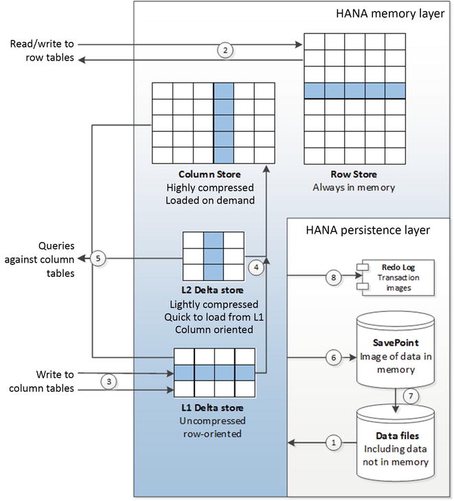
Figure 7-7. SAP HANA architecture
Again, we see that although HANA is described as an in-memory database, there are situations in which an application will need to wait for IO from a disk device; that is, on commit, and when column tables are loaded on demand into memory.
Redis, HANA, and TimesTen are legitimate in-memory database systems: designed from the ground up to use memory as the primary—and usually exclusive—source for all data. However, as we have seen, applications that use these systems still often need to wait for disk IO. In particular, there will often be a disk IO to some form of journal or transaction log when a transaction commits.
VoltDB is a commercial implementation of the H-store design. H-store was one of the databases described in Michael Stonebraker’s seminal 2007 paper, which argued that no single database architecture was suitable for all modern workloads.1 H-store describes an in-memory database designed with the explicit intention of not requiring disk IO during normal transactional operations—it aspires to be a pure in-memory solution.
VoltDB supports the ACID transactional model, but rather than guaranteeing data persistence by writing to a disk, persistence is guaranteed through replication across multiple machines. A transaction commit only completes once the data is successfully written to memory on more than one physical machine. The number of machines involved depends on the K-safety level specified. For instance, a K-safety level of 2 guarantees no data loss if any two machines fail; in this case, the commit must successfully be propagated to three machines before completing.
It is also possible to configure a command log that records transaction commands in a disk-based log. This log may be synchronous—written to at every transaction commit —or asynchronous. Because VoltDB supports only deterministic stored procedure-based transactions, the log need only record the actual command that drove the transaction, rather than copies of modified blocks, as is common in other database transaction logs. Nonetheless, if the synchronous command logging option is employed, then VoltDB applications may experience disk IO wait time.
VoltDB supports the relational model, though its clustering scheme works best if that model can be partitioned hierarchically across common keys. In VoltDB, tables must either be partitioned or replicated. Partitions are distributed across nodes of the cluster while replicated tables are duplicated in each partition. Tables that are replicated may incur additional overhead during OLTP operations, since the transactions must be duplicated in each partition; this is in contrast to partitioned tables, which incur additional overhead if data must be collated from multiple partitions. For this reason, replicated tables are usually smaller reference-type tables, while the larger transactional tables are partitioned.
Partitions in VoltDB are distributed not just across physical machines but also within machines that have multiple CPU cores. In VoltDB, each partition is dedicated to a single CPU that has exclusive single-threaded access to that partition. This exclusive access reduces the overhead of locking and latching, but it does require that transactions complete quickly to avoid serialization of requests.
Figure 7-8 illustrates how partitioning and replication affect concurrency in VoltDB. Each partition is associated with a single CPU core, and only one SQL statement will ever be active against the partition at any given moment (1). In this example, ORDERS and CUSTOMERS have been partitioned using the customer ID, while the PRODUCTS table is replicated in its entirety in all partitions. A query that accesses data for a single customer need involve only a single partition (2), while a query that works across customers must access—exclusively, albeit for a short time—all partitions (3).

Figure 7-8. VoltDB partitioning
VoltDB transactions are streamlined by being encapsulated into a single Java stored procedure call, rather than being represented by a collection of separate SQL statements. This ensures that transaction durations are minimized (no think-time or network time within transactions) and further reduces locking issues.
Oracle 12c “in-Memory Database”
Oracle RDBMS version 12.1 introduced the “Oracle database in-memory” feature. This wording is potentially misleading, since the database as a whole is not held in memory. Rather, Oracle has implemented an in-memory column store to supplement its disk-based row store.
Figure 7-9 illustrates the essential elements of the Oracle in-memory column store architecture. OLTP applications work with the database in the usual manner. Data is maintained in disk files (1), but cached in memory (2). An OLTP application primarily reads and writes from memory (3), but any committed transactions are written immediately to the transaction log on disk (4). When required or as configured, row data is loaded into a columnar representation for use by analytic applications (5). Any transactions that are committed once the data is loaded into columnar format are recorded in a journal (6), and analytic queries will consult the journal to determine if they need to read updated data from the row store (7) or possibly rebuild the columnar structure.

Figure 7-9. Oracle 12c “in-memory” architecture
Berkeley Analytics Data Stack and Spark
If SAP HANA and Oracle TimesTen represent in-memory variations on the relational database theme, and if Redis represents an in-memory variation on the key-value store theme, then Spark represents an in-memory variation on the Hadoop theme.
Hadoop became the de facto foundation for today’s Big Data stack by providing a flexible, scalable, and economic framework for processing massive amounts of structured, unstructured, and semi-structured data. The Hadoop 1.0 MapReduce algorithm represented a relatively simple but scalable approach to parallel processing. MapReduce is not the most elegant or sophisticated approach for all workloads, but it can be adapted to almost any problem, and it can usually scale through the brute-force application of many servers.
However, it’s long been realized that MapReduce—particularly when working on disk-based storage—is not a sufficient solution for emerging Big Data analytic challenges. MapReduce excels at batch processing, but falls short in real-time scenarios. Even the simplest MapReduce task takes a significant ramp-up time, and for some machine-learning algorithms the execution time is simply inadequate.
In 2011, the AMPlab (Algorithms, Machines, and People) was established at University of California, Berkeley, to attack the emerging challenges of advanced analytics and machine learning on Big Data. The resulting Berkeley Data Analysis Stack (BDAS)—and in particular the Spark processing engine—has shown rapid uptake.
BDAS consists of a few core components:
- Spark is an in-memory, distributed, fault-tolerant processing framework. Implemented in the Java virtual-machine-compatible programming language Scala, it provides higher-level abstractions than MapReduce and thus improves developer productivity. As an in-memory solution, Spark excels at tasks that cause bottlenecks on disk IO in MapReduce. In particular, tasks that iterate repeatedly over a dataset—typical of many machine-learning workloads—show significant improvements.
- Mesos is a cluster management layer somewhat analogous to Hadoop’s YARN. However, Mesos is specifically intended to allow multiple frameworks, including BDAS and Hadoop, to share a cluster.
- Tachyon is a fault-tolerant, Hadoop-compatible, memory-centric distributed file system. The file system allows for disk storage of large datasets, but promotes aggressive caching to provide memory-level response times for frequently accessed data.
Other BDAS components build on top of this core. Spark SQL provides a Spark-specific implementation of SQL for ad hoc queries, and there is also an active effort to allow Hive— the SQL implementation in the Hadoop stack—to generate Spark code.
Spark streaming provides a stream-oriented processing paradigm using the Spark foundation, and GraphX delivers a graph computation engine build on Spark. BDAS also delivers machine-learning libraries at various levels of abstraction in the MLBase component.
Spark is sometimes referred to as a successor to Hadoop, but in reality Spark and other elements of the BDAS were designed to work closely with Hadoop HDFS and YARN, and many Spark implementations use HDFS for persistent storage. Figure 7-10 shows how Hadoop elements such as YARN and HDFS interact with Spark and other elements of the BDAS.

Figure 7-10. Spark, Hadoop, and the Berkeley Data Analytics Stack
Spark is incorporated into many other data management stacks; it is a core part of the three major organizational distributions of Hadoop (Cloudera, Hortonworks, and MapR). Spark is also a component of the Datastax distribution of Cassandra.
In Spark, data is represented as resilient distributed datasets (RDD). RDDs are collections of objects that can be partitioned across multiple nodes of the cluster. The partitioning and subsequent distribution of processing are handled automatically by the Spark framework.
RDDs are described as immutable: Spark operations on RDDs return new RDDs, rather than modifying the original RDD. So, for instance, sorting an RDD creates a new RDD that contains the sorted data.
The Spark API defines high-level methods that perform operations on RDDs. Operations such as joining, filtering, and aggregation, which would entail hundreds of lines of Java code in MapReduce, are expressed as simple method calls in Spark; the level of abstraction is similar to that found with Hadoop’s Pig scripting language.
The data within an RDD can be simple types such as strings or any other Java/Scala object type. However, it’s common for the RDD to contain key-value pairs, and Spark provides specific data manipulation operations such as aggregation and joins that work only on key-value oriented RDDs.
Under the hood, Spark RDD methods are implemented by directed acyclic graph (DAG) operations. Directed acyclic graphs provide a more sophisticated and efficient processing paradigm for data manipulation than MapReduce. We discuss directed acyclic graph operations in Chapter 11.
Although Spark expects data to be processed in memory, Spark is capable of managing collections of data that won’t fit entirely into main memory. Depending on the configuration, Spark may page data to disk if the data volumes exceed memory capacity.
Spark is not an OLTP-oriented system, so there is no need for the transaction log or journal that we’ve seen in other in-memory databases. However, Spark can read from or write to local or distributed file systems, and in particular it integrates with the standard Hadoop methods for working with HDFS or external data. RDDs may be represented on disk as text files or JSON documents.
Spark can also access data held in any JDBC-compliant database (in practice, almost every relational system), as well as from HBase or Cassandra.
Figure 7-11 illustrates some of the essential features of Spark processing. Data can be loaded into resilient distributed datasets (RDD) from external sources including relational databases (1) or a distributed file system such as HDFS (2). Spark provides high-level methods for operating on RDDs and which output new RDDs. These operations include joins (3) or aggregations (4). Spark data may be persisted to disk in a variety of formats (5).

Figure 7-11. Elements of Spark processing
Conclusion
It’s definitely premature to predict the end of magnetic disks in database systems: magnetic disks still offer the best economics for storage of massive amounts of “cold” or “warm” data, and in the age of Big Data the economics of storage still matter. However, solid state disk provides better economics for datasets where the speed of retrieval is more important than the cost of long-term storage. And all significant database systems are adapting to the unique physical characteristics of SSD. Some databases are being built from the ground up to exploit SSD processing characteristics.
As memory reduces in price, and the amount of memory that can be housed in a single database server increases, in-memory architectures grow ever more attractive for databases of smaller size or where latency or transaction processing speed are more important than economics of mass storage. When a database cannot fit into the memory of a single server, a distributed in-memory system may offer a compelling high-performance solution.
We’ve seen how in-memory database designs have arisen in each category of database system: relational, key-value, and Big Data. There are also an increasing number of hybrid designs such as Oracle’s, which attempt to merge the processing benefits of an in-memory approach with the storage economics that are still only provided by traditional disk devices.
Note
- The End of an Architectural Era (It’s Time for a Complete Rewrite), http://nms.csail.mit.edu/~stavros/pubs/hstore.pdf