
![]()
Data Models and Storage
A model’s just an imitation of the real thing.
—Mae West
The ocean flows of online information are all streaming together, and the access tools are becoming absolutely critical. If you don’t index it, it doesn’t exist. It’s out there but you can’t find it, so it might as well not be there.
—Barbara Quint
The relational database model provided a strong theoretical foundation for the representation of data that eliminated redundancy and maximized flexibility of data access. Many next-generation database systems, particularly those of the NewSQL variety, continue to embrace the relational model: their innovations generally focus on the underlying physical storage of data.
However, databases of the NoSQL variety explicitly reject the fixed schema of the relational model. This rejection is not based on any theoretical disagreement with the principles of relational data modeling but, rather, from a practical desire to facilitate agility in application development by allowing schemas to evolve with the application. Additionally, NoSQL databases seek to avoid the overhead created by operations such as joins, which are a necessary consequence of relational normalization.
Underneath the data model, all databases adopt physical storage mechanisms designed to optimize typical access paths. Following our review of new and traditional data models in this chapter, we’ll examine how storage is designed to support the models.
Today’s databases adopt a variety of data models:
- Relational models serve as the inspiration for the representation of data in the traditional RDBMS (Oracle, SQL Server, etc.), as well as for NewSQL databases such as Vertica and VoltDB.
- Key-value stores theoretically impose no structure or limitation on the “value” part of the key value. However, in practice, most key-value stores provide additional support for certain types of data structures to allow for indexing and conflict resolution.
- Databases based on Google’s BigTable database implement the wide column store described in the BigTable specification. However, some significant innovations have been introduced in databases such as Cassandra.
- Document databases use JSON or XML documents, which generally impose no restriction on the data that can be represented, but which provide a self-describing and predictable data representation.
- Graph databases represent data as nodes, relationships, and properties. Graph databases were described in detail in Chapter 5.
Review of the Relational Model of Data
Before diving into nonrelational data models, let’s quickly recapitulate the relational model, which dominated the last generation of database systems and which remains the most widely adopted data model today. The relational model forms the basis not just for the traditional RDBMS but also for databases of the NewSQL variety—databases such as Vertica and VoltDB, for instance. We provided an overview of the relational model back in Chapter 1, and of course the relational data model is supported by a vast body of literature. What follows is a brief summary.
The relational model organizes values into tuples (rows). Multiple tuples are used to construct relations (tables). Rows are identified by key values and—at least in third normal form—all values will be locatable by the entire primary key and nothing else. Foreign keys define relationships between tables by referencing the primary keys in another table.
The process of eliminating redundancy from a relational model is known as normalization. Figure 10-1 provides an example of un-normalized and normalized data.

Figure 10-1. Normalized relational data model
The star schema represents a data modeling pattern commonly found—indeed, almost always found—in data warehouses. In a star schema, a large “fact” table contains detailed business data and contains foreign keys to smaller more static “dimension” tables that categorize the fact items in business terms, typically including time, product, customer, and so on.
Figure 10-2 shows an example of a star schema. The central SALES fact table contains sales totals that are aggregated across various time periods, products, and customers. The detail and explanation of each aggregation can be found by joining to the dimension tables TIMES, PRODUCTS, and CUSTOMERS.

Figure 10-2. Star schema
Unlike the relational model, there is no formal definition for how data is represented in a key-value store. Typically a key-value store will accept any binary value within specific size limits as a key and is capable of storing any binary data as a value. In this respect, we might say that the key-value store is data-type agnostic. However, most key-value stores provide additional support for certain types of data. The support stems from the desire to provide one of the following features:
- Secondary indexes. In a pure key-value store, the only way to locate an object is via its key. However, most applications perform lookups on non-key terms. For instance, we may wish to locate all users within a geography, all orders for a specific company, and so on.
- Conflict resolution. Key-value stores that provide eventual consistency or Amazon Dynamostyle tunable consistency may implement special data types that facilitate conflict resolution.
Riak, a key-value store based on Amazon’s Dynamo specification, illustrates both of these patterns.
As well as binary objects, Riak allows for data to be defined as one of the following:
- A Riak convergent replicated data type (CRDT). These data types, described in more detail below, include maps, sets, and counters. Conflicting operations on these data types can be resolved by Riak without requiring application or human intervention.
- A document type, such as XML, JSON, or Text.
- A custom data type.
Riak includes Solr, an open-source text search engine. When a Riak value is defined as one of the built-in data types, or as a custom data type for which you have provided custom search code, then Solr will index the value and provide a variety of lookup features, including exact match, regular expression, and range searches.
In the case of JSON, XML, and Riak maps, searches can be restricted to specific fields within the document. So, for instance, you could search for documents that have a specific value for a specific JSON attribute.
Convergent Replicated Data Types
We touched on convergent replicated data types (CRDT) in Chapter 9. As we noted there, Riak users vector clocks to determine if two updates potentially conflict. By default, if after the examination of the vector clocks for two conflicting updates the system cannot determine which of the updates is most correct, then Riak will maintain both versions of the update by creating sibling values, which must be resolved by the user or application.
CRDTs allow two conflicting updates to be merged even if their vector clocks indicate that they are concurrent. A CRDT encapsulates deterministic rules that can be used either to merge the conflicting values or to determine which of two conflicting values should “win” and be propagated.
When a CRDT value is propagated between nodes, it includes not just the current value of the object but also a history of operations that have been applied to the object. This history is somewhat analogous to the vector clock data that accompanies each update in a Riak system, but unlike a vector clock, it contains information specifically pertaining to the history of a specific object.
The simplest example of CRDT merging involves the g-counter (grow-only counter) data type. This is a monotonically incrementing counter that cannot be decremented (e.g., you can increase the counter, but you cannot decrease its value).
You might think that you could merge g-counter updates simply by adding up all the increment operations that have occurred on every node to determine the total counter value. However, this approach ignores the possibility that some of these increment operations are replicas of other increment operations. To avoid such double counting, each node maintains an array of the counter values received from every node. Upon incrementing, the node increments its element in the array and then transmits the entire array to other nodes. Should a conflict between updates be detected (through the vector clock mechanism), we take the highest element for each node in each version and add them up.
That last sentence was quite a mouthful, but it’s still simpler than the mathematical notation! Stepping through the example shown in Figure 10-3 will, we hope, illuminate the process.
- At time t0, each node has a value of 0 for the counter, and each element in the array of counters (one for each node) is also set to 0.
- Around time t1, node 1 receives an increment operation on the counter of +1, while node 2 receives an increment operation of +2. Nodes 1 and 2 transmit their counter values to node 3.
- Around time t2, node 1 receives an increment of +4 and an update from node 2, while node 3 receives an increment of +2. Each node now has a different value for the counter: 7 (5,0,2), 3 (1,0,2), or 4 (0,0,4).
- Around time t3, node 2 receives updates from node 1 and node 3. These updates are potentially conflicting, so node 2 has to merge the three counter arrays. By taking the highest element for each node from each array, node 2 concludes that the correct value for the counter is (5,0,4), which adds up to 9.
- At time t4, node 2 propagates the correct values of the counter to the other nodes and the cluster is now back in sync.

Figure 10-3. Convergent replicated data type g-counter
Other CRDTs are defined in academia and implemented in Riak or in other databases. For instance:
- The PN-counter type allows counters to increment and decrement safely. It is implemented as two g-counters, one which maintains increments and the other which maintains decrements.
- The G-set type implements a collection of objects to which you can add elements but never remove them.
- The 2P-set provides a collection to which elements can be removed as well as inserted. However, an object can be removed only once.
- The LWW-set allows multiple insertions and deletes, with a last-write-wins policy in the event of conflicting operations.
Other CRDT types provide further flexibility in the operations they support, but in a manner similar to the LWW-set type, specify winners and losers in the event of conflict. The winner might be determined by timestamps or by comparing the relative number of operations to which the element has been subjected, or by some other domain-specific logic.
Data Models in BigTable and HBase
Google’s BigTable paper was published in 2006 and was the basis for the data model used in HBase, Cassandra, and several other databases. Google also makes BigTable storage available as a service in the Google Cloud BigTable product.
BigTable tables have the following characteristics:
- Data is organized as tables that—like relational tables—have columns and rows.
- Tables are indexed and sorted by a single rowkey.
- A table includes one or more column families, which are named and specified in the table definition.
- Column families are composed of columns. Column names are dynamic, and new columns can be created dynamically upon insertion of a new value. Use of the term “column” is somewhat misleading: BigTable column families are more accurately described as sorted multidimensional maps, in which values are identified by column name and timestamp.
- Data for a specific column family is stored together on disk.
- Tables are sparse: empty columns do not take up space.
- A cell (intersection of row and column) may contain multiple versions of a data element, indexed by timestamp.
Column families can be used to group related columns for convenience, to optimize disk IO by co-locating columns that are frequently accessed together on disk, or to create a multidimensional structure that can be used for more complex data.
Figure 10-4 illustrates a simple column family structure. Rows are grouped into three column families, but each row has identical column names. In this configuration, the table resembles a relational table that has been vertically partitioned on disk for performance reasons.
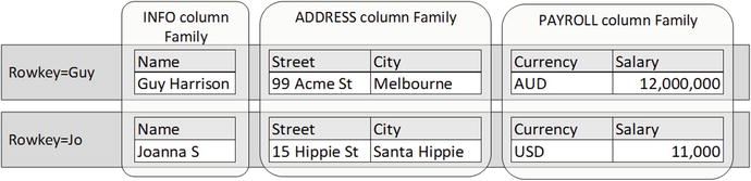
Figure 10-4. Simple column family structure
The uniqueness of the BigTable data model becomes more apparent when we create a “wide” column family. In this case, column names represent the name portion of a name:value pair. Any given row key may have any arbitrary collection of such columns, and there need be no commonality between rowkeys with respect of column names.
Figure 10-5 illustrates such a wide column family. In the FRIENDS column family, we have a variable number of columns, each corresponding to a specific friend. The name of the column corresponds to the name of the friend, while the value of the column is the friend’s email. In this example, both Guy and Joanna have a common friend John, so each share that column. But other columns that represent friends who are not shared, and those columns appear only in the row required.

Figure 10-5. Wide column family structure
BigTable/HBase column families are described as sparse because no storage is consumed by columns that are absent in a given row. Indeed, a BigTable column family is essentially a “map” consisting of an arbitrary set of sorted name:value pairs.
Versions
Each cell in a BigTable column family can store multiple versions of a value, indexed by timestamp. Timestamps may be specified by the application or automatically assigned by the server. Values are stored within a cell in descending timestamp order, so by default a read will retrieve the most recent timestamp. A read operation can specify a timestamp range or specify the number of versions of data to return.
A column family configuration setting specifies the maximum number of versions that will be stored for each value. In HBase, the default number of versions is three. There is also a minimum version count, which is typically combined with a time to live (TTL) setting. The TTL setting instructs the server to delete values that are older than a certain number of seconds. The minimum version count overrides the TTL, so typically at least one or more copies of the data will be kept regardless of age.
Figure 10-6 illustrates multiple values with timestamps. For the row shown, the info:loc column has only a single value, but the readings:temp column has five values corresponding perhaps to the last five readings of a thermostat.

Figure 10-6. Multiple versions of cell data in BigTable
Deletes in a BigTable database are implemented by creating tombstone markers that indicate all versions of a column or column family less than a given timestamp have been removed. By default, a delete uses the current timestamp, thus eliminating all previous row values.
Deleted elements persist on disk until a compaction occurs. We’ll discuss compaction later in this chapter.
Cassandra
Cassandra’s data model is based on the BigTable design, but has evolved significantly since its initial release. Indeed, it can be hard to recognize the BigTable structure when working with Cassandra through the Cassandra Query Language (CQL).
The CQL CREATE TABLE statement allows us to define composite primary keys, which look like familiar multi-column keys in relational databases. For instance, in the CQL shown below, we create a table FRIENDS, which is keyed on columns NAME and FRIEND corresponding to the user’s name and the name of each of his or her friends:
CREATE TABLE friends
 (user text,
  friend text,
  email text,
PRIMARY KEY (user,friend));
CQL queries on this table return results that imply one row exists for each combination of user and friend:
cqlsh:guy>   SELECT * FROM friends;

 user | friend | email
------+--------+------------------
   Jo | George | [email protected]
   Jo |    Guy |    [email protected]
   Jo |   John |   [email protected]
  Guy |     Jo |     Jo@gmail.com
But when we look at the column family using the (now depreciated) thrift client, we can see we have two rows, one with four columns and the other with six columns (the output here has been edited for clarity):
RowKey: Jo
=> (name=George:,      value=,                 timestamp=...)
=> (name=George:email, value[email protected], timestamp=...)
=> (name=Guy:,         value=,                 timestamp=...)
=> (name=Guy:email,    value[email protected],    timestamp=...)
=> (name=John:,        value=,                 timestamp=...)
=> (name=John:email,   value[email protected],   timestamp=...)
-------------------
RowKey: Guy
=> (name=Jo:,          value=,                 timestamp=...)
=> (name=Jo:email,     value[email protected],     timestamp=...)
=> (name=John:,        value=,                 timestamp=...)
=> (name=John:email,   value[email protected],   timestamp=...)

2 Rows Returned.
The first part of the CQL primary key (USER, in our example) is used to specify the rowkey for the table and is referred to as the partition key. The second parts of the primary key (FRIEND, in our example) are clustering keys and are used to create a wide column structure in which each distinct value of the CQL key column is used as part of the name of a BigTable-style column. So for instance, the column Guy:email is constructed from the value “Guy” within the CQL column “Friend” together with the name of the CQL column “email.”
That’s quite confusing! So it’s no wonder that Cassandra tends to hide this complexity within a more familiar relational style SQL-like notation. Figure 10-7 compares the Cassandra CQL representation of the data with the underlying BigTable structure: the apparent five rows as shown in CQL are actually implemented as two BigTable-style rows in underlying storage.

Figure 10-7. Cassandra CQL represents wide column structure as narrow tables
![]() Note Cassandra uses the term “column family” differently from HBase and BigTable. A Cassandra column family is equivalent to a table in HBase. For consistency’s sake, we may refer to Cassandra “tables” when a Cassandra purist would say “column family.”
Note Cassandra uses the term “column family” differently from HBase and BigTable. A Cassandra column family is equivalent to a table in HBase. For consistency’s sake, we may refer to Cassandra “tables” when a Cassandra purist would say “column family.”
The underlying physical implementation of Cassandra tables explains some of the specific behaviors within the Cassandra Query Language. For instance, CQL requires that an ORDER BY clause refer only to composite key columns. WHERE clauses in CQL also have restrictions that seem weird and arbitrary unless you understand the underlying storage model. The partition key accepts only equality clauses (IN and “=”), which makes sense when you remember that rowkeys are hash-partitioned across the cluster, as we discussed in Chapter 8. Clustering key columns do support range operators such as “>” and “<”, which again makes sense when you remember that in the BigTable model the column families are actually sorted hash maps.
Cassandra Collections
Cassandra’s partitioning and clustering keys implement a highly scalable and efficient storage model. However, Cassandra also supports collection data types that allow repeating groups to be stored within column values.
For instance, we might have implemented our FRIENDS table using the MAP data type, which would have allowed us to store a hash map of friends and emails within a single Cassandra column:
CREATE TABLE friends2
 (person text,
  friends map<text,text>,
  PRIMARY KEY (person ));

  INSERT into friends2(person,friends)
  VALUES('Guy',
         {'Jo':'[email protected]',
          'john':'[email protected]',
          'Chris':'[email protected]'});
Cassandra also supports SET and LIST types, as well as the MAP type shown above.
JSON Data Models
JavaScript Object Notation (JSON) is the de facto standard data model for document databases. We devoted Chapter 4 to document databases; here, we will just formally look at some of the elements of JSON.
JSON documents are built up from a small set of very simple constructs: values, objects, and arrays.
- Arrays consist of lists of values enclosed by square brackets (“[“ and “]”) and separated by commas (“,”).
- Objects consist of one or more name value pairs in the format “name”:”value” , enclosed by braces (“{“ and ”}” ) and separated by commas (“,”).
- Values can be Unicode strings, standard format numbers (possibly including scientific notation), Booleans, arrays, or objects.
The last few words in the definition are very important: because values may include objects or arrays, which themselves contain values, a JSON structure can represent an arbitrarily complex and nested set of information. In particular, arrays can be used to represent repeating groups of documents, which in a relational database would require a separate table.
Document databases such as CouchBase and MongoDB organize documents into buckets or collections, which would generally be expected to contain documents of a similar type. Figure 10-8 illustrates some of the essential JSON elements.

Figure 10-8. JSON documents
MongoDB stores JSON documents internally in the BSON format. BSON is designed to be a more compact and efficient representation of JSON data, and it uses more efficient encoding for numbers and other data types. In addition, BSON includes field length prefixes that allow scanning operations to “skip over” elements and hence improve efficiency.
Storage
One of the fundamental innovations in the relational database model was the separation of logical data representation from the physical storage model. Prior to the relational model it was necessary to understand the physical storage of data in order to navigate the database. That strict separation has allowed the relational representation of data to remain relatively static for a generation of computer scientists, while underlying storage mechanisms such as indexing have seen significant innovation. The most extreme example of this decoupling can be seen in the columnar database world. Columnar databases such as Vertica and Sybase IQ continue to support the row-oriented relational database model, even while they have tipped the data on its side by storing data in a columnar format.
We have looked at the underlying physical storage of columnar systems in Chapter 6, so we don’t need to examine that particular innovation here. However, there has been a fundamental shift in the physical layout of modern nonrelational databases such as HBase and Cassandra. This is the shift away from B-tree storage structure optimized for random access to the log-structured Merge tree pattern, which is optimized instead for sequential write performance.
Typical Relational Storage Model
Most relational databases share a similar high-level storage architecture.
Figure 10-9 shows a simplified relational database architecture. Database clients interact with the database by sending SQL to database processes (1). The database processes retrieve data from database files on disk initially (2), and store the data in memory buffers to optimize subsequent accesses (3). If data is modified, it is changed within the in-memory copy (4). Upon transaction commit, the database process writes to a transaction log (5), which ensures that the transaction will not be lost in the event of a system failure. The modified data in memory is written out to database files asynchronously by a “lazy” database writer process (6).

Figure 10-9. Relational database storage architecture
Much of the architecture shown in Figure 10-9 can be found in nonrelational systems as well. In particular, some equivalent of the transaction log is present in almost any transactional database system.
Another ubiquitous RDBMS architectural pattern—at least in the operational database world—is the B-tree index. The B-tree index is a structure that allows for random access to elements within a database system.
Figure 10-10 shows a B-tree index structure. The B-tree index has a hierarchical tree structure. At the top of the tree is the header block. This block contains pointers to the appropriate branch block for any given range of key values. The branch block will usually point to the appropriate leaf block for a more specific range or, for a larger index, point to another branch block. The leaf block contains a list of key values and the physical addresses of matching table data.

Figure 10-10. B-tree index structure
Leaf blocks contain links to both the previous and the next leaf block. This allows us to scan the index in either ascending or descending order, and allows range queries using the “>”, “<” or “BETWEEN” operators to be satisfied using the index.
B-tree indexes offer predictable performance because every leaf node is at the same depth. Each additional layer in the index exponentially increases the number of keys that can be supported, and for almost all tables, three or four IOs will be sufficient to locate any row.
However, maintaining the B-tree when changing data can be expensive. For instance, consider inserting a row with the key value “NIVEN” into the table index diagrammed in Figure 10-10. To insert the row, we must add a new entry into the L-O block. If there is no free space within a leaf block for a new entry, then an index split is required. A new block must be allocated and half of the entries in the existing block have to be moved into the new block. As well as this, there is a requirement to add a new entry to the branch block (in order to point to the newly created leaf block). If there is no free space in the branch block, then the branch block must also be split.
These index splits are an expensive operation: new blocks must be allocated and index entries moved from one block to another, and during this split access times will suffer. So although the B-tree index is an efficient random read mechanism, it is not so great for write-intensive workloads.
The inherent limitations of the B-tree structure are somewhat mitigated by the ability to defer disk writes to the main database files: as long as a transaction log entry has been written on commit, data file modifications—including index blocks—can be performed in memory and written to disk later. However, during periods of heavy, intensive write activity, free memory will be exhausted and throughput will be limited by disk IO to the database blocks.
There have been some significant variations on the B-tree pattern to provide for better throughput for write-intensive workloads: Both Couchbase’s HB+-Trie and Tokutek’s fractal tree index claim to provide better write optimization.
However, an increasing number of databases implement a storage architecture that is optimized from the ground up to support write-intensive workloads: the log-structured merge (LSM) tree.
Log-structured Merge Trees
The log-structured merge (LSM) tree is a structure that seeks to optimize storage and support extremely high insert rates, while still supporting efficient random read access.
The simplest possible LSM tree consists of two indexed “trees”:
- An in–memory tree, which is the recipient of all new record inserts. In Cassandra, this in-memory tree is referred to as the MemTable and in HBase as the MemStore.
- A number of on-disk trees, which represent copies of in-memory trees that have been flushed to disk. In Cassandra, this on-disk structure is referred to as the SSTable and in HBase as the StoreTable.
The on-disk tree files are initially point-in-time copies of the in-memory tree, but are merged periodically to create larger consolidated stores. This merging process is called compaction.
![]() Note The log-structured merge tree is a very widely adopted architecture and is fundamental to BigTable, HBase, Cassandra, and other databases. However, naming conventions vary among implementations. For convenience, we use the Cassandra terminology by default, in which the in-memory tree is called a MemTable and the on-disk trees are called SSTables.
Note The log-structured merge tree is a very widely adopted architecture and is fundamental to BigTable, HBase, Cassandra, and other databases. However, naming conventions vary among implementations. For convenience, we use the Cassandra terminology by default, in which the in-memory tree is called a MemTable and the on-disk trees are called SSTables.
The LSM architecture ensures that writes are always fast, since they operate at memory speed. The transfer to disk is also fast, since it occurs in append-only batches that allow for fast sequential writes. Reads occur either from the in-memory tree or from the disk tree; in either case, reads are facilitated by an index and are relatively swift.
Of course, if the server failed while data was in the in-memory store, then it could be lost. For this reason database implementations of the LSM pattern include some form of transaction logging so that the changes can be recovered in the event of failure. This log file is roughly equivalent to a relational database transaction (redo) log. In Cassandra, it is called the CommitLog and in HBase, the Write-Ahead Log (WAL). These log entries can be discarded once the in-memory tree is flushed to disk.
Figure 10-11 illustrates the log-structured merge tree architecture, using Cassandra terminology. Writes from database clients are first applied to the CommitLog (1) and then to the MemTable (2). Once the MemTable reaches a certain size, it is flushed to disk to create a new SSTable (3). Once the flush completes, CommitLog records may be purged (4). Periodically, multiple SSTables are merged (compacted) into larger SSTables (5).

Figure 10-11. LSM architecture (Cassandra terminology)
The on-disk portion of the LSM tree is an indexed structure. For instance, in Cassandra, each SSTable is associated with an index that contains all the rowkeys that exist in the SSTable and an offset to the location of the associated value within the file. However, there may be many SSTables on disk, and this creates a multiplier effect on index lookups, since we would theoretically have to examine every index for every SSTable in order to find our desired row.
To avoid these multiple-index lookups, bloom filters are used to reduce the number of lookups that must be performed.
Bloom filters are created by applying multiple hash functions to the key value. The outputs of the hash functions are used to set bits within the bloom filter structure. When looking up a key value within the bloom filter, we perform the same hash functions and see if the bits are set. If the bits are not set, then the search value must not be included within the table. However, if the bits are set, it may have been as a result of a value that happened to hash to the same values. The end result is an index that is typically reduced in size by 85 percent, but that provides false positives only 15 percent of the time.
Bloom filters are compact enough to fit into memory and are very quick to navigate. However, to achieve this compression, bloom filters are “fuzzy” in the sense that they may return false positives. If you get a positive result from a bloom filter, it means only that the file may contain the value. However, the bloom filter will never incorrectly advise you that a value is not present. So if a bloom filter tells us that a key is not included in a specific SSTable, then we can safely omit that SSTable from our lookup.
Figure 10-12 shows the read pattern for a log-structured merge tree using Cassandra terminology. A database request first reads from the MemTable (1). If the required value is not found, it will consult the bloom filters for the most recent SSTable (2). If the bloom filter indicates that no matching value is present, it will examine the next SSTable (3). If the bloom filter indicates a matching key value may be present in the SSTable, then the process will use the SSTable index (4) to search for the value within the SSTable (5). Once a matching value is found, no older SSTables need be examined.

Figure 10-12. Log-structured merge tree reads (Cassandra terminology)
SSTables are immutable—that is, once the MemTable is flushed to disk and becomes an SSTable, no further modifications to the SSTable can be performed. If a value is modified repeatedly over a period of time, the modifications will build up across multiple SSTables. When retrieving a value, the system will read SSTables from the youngest to the oldest to find the most recent value of a column, or to build up a complete row. Therefore, to update a value we need only insert the new value, since the older values will not be examined when a newer version exists.
Deletions are implemented by writing tombstone markers into the MemTable, which eventually propagates to SSTables. Once a tombstone marker for a row is encountered, the system stops examining older entries and reports “row not found” to the application.
As SSTables multiply, read performance and storage degrade as the numbers of bloom filters, indexes, and obsolete values increase. So periodically the system will compact multiple SSTables into a single file. During compaction, rows that are fragmented across multiple SSTables are consolidated and deleted rows are removed.
However, tombstones will remain in the system for a period of time to ensure that a delayed update to a row will not resurrect a row that should remain deleted. This can happen if a tombstone is removed while older updates to that row are still being propagated through the system. To avoid this possibility, default settings prevent tombstones from being deleted for over a week, while hinted handoffs (see Chapter 8) generally expire after only three hours. But in the event of these defaults being adjusted, or in the event of an unreasonably long network partition, it is conceivable that a row that has been deleted will be resurrected.
A secondary index allows us to quickly find rows that meet some criteria other than their primary key or rowkey value.
Secondary indexes are ubiquitous in relational systems: it’s a fundamental characteristic of a relational system that you be able to navigate primary key and foreign key relationships, and this would be impractical if only primary key indexes existed. In relational systems, primary key indexes and secondary indexes are usually implemented in the same way: most commonly with B-tree indexes, or sometimes with bitmap indexes.
We discussed in Chapter 6 how columnar databases often use projections as an alternative to indexes: this approach works in columnar systems because queries typically aggregate data across a large number of rows rather than seeking a small number of rows matching a specific criteria. We also discussed in Chapter 5 how graph databases use index-free adjacency to perform efficient graph traversal without requiring a separate index structure.
Neither of these solutions are suitable for nonrelational operational database systems. The underlying design of key-value stores, BigTable systems, and document databases assumes data retrieval by a specific key value, and indeed in many cases—especially in earlier key-value systems—lookup by rowkey value is the only way to find a row.
However, for most applications, fast access to data by primary key alone is not enough. So most nonrelational databases provide some form of secondary index support, or at least provide patterns for “do-it-yourself” secondary indexing.
Creating a secondary index for a key-value store is conceptually fairly simple. You create a table in which the key value is the column or attribute to be indexed, and that contains the rowkey for the primary table.
Figure 10-13 illustrates the technique. The table USERS contains a unique identifier (the rowkey) for each user, but we often want to retrieve users by email address. Therefore, we create a separate table in which the primary key is the user’s email address and that contains the rowkey for the source table.

Figure 10-13. Do-it-yourself secondary indexing
Variations on the theme allow for indexing of non-unique values. For instance, in a wide column store such as HBase, an index entry might consist of multiple columns that point to the rows matching the common value as shown in the “COUNTRY” index in Figure 10-13.
However, there are some significant problems with the do-it-yourself approach outlined above:
- It’s up to the application code to consistently maintain both the data in the base table and all of its indexes. Bugs in application code or ad hoc manipulation of data using alternative clients can lead to missing or incorrect data in the index.
- Ideally, the operations that modify the base table and the operation that modifies the index will be atomic: either both succeed or neither succeeds. However, in nonrelational databases, multi-object transactions are rarely available. If the index operation succeeds but not the base table modification (or vice versa), then the index will be incorrect.
- Eventual consistency raises a similar issue: an application may read from the index an entry that has not yet been propagated to every replica of the base table (or vice versa).
- The index table supports equality lookups, but generally not range operations, since unlike as in the B-tree structure, there is no pointer from one index entry to the next logical entry.
Do-it-yourself indexing is not completely impractical, but it places a heavy burden on the application and leads in practice to unreliable and fragile implementations. Most of these issues are mitigated when a database implements a native secondary indexing scheme. The secondary index implementation can be made independent of the application code, and the database engine can ensure that index entries and base table entries are maintained consistently.
Distributed databases raise additional issues for indexing schemes. If index entries are partitioned using normal mechanisms—either by consistent hashing of the key value or by using the key value as a shard key—then the index entry for a base table row is typically going to be located on a different node. As a result, most lookups will usually span two nodes and hence require two IO operations.
If the indexed value is unique, then the usual sharding or hashing mechanisms will distribute data evenly across the cluster. However, if the key value is non-unique, and especially if there is significant skew in the distribution of values, then index entries and hence index load may be unevenly distributed. For instance, the index on COUNTRY in Figure 10-13 would result in the index entries for the largest country (USA, in our example) being located on a single node.
To avoid these issues, secondary indexes in nonrelational databases are usually implemented as local indexes. Each node maintains its own index, which references data held only on the local node. Index-dependent queries are issued to each node, which returns any matching data via its local index to the query coordinator, which combines the results.
Figure 10-14 illustrates the local secondary indexing approach. A database client requests data for a specific non-key value (1). A query coordinator sends these requests to each node in the cluster (2). Each node examines its local index to determine if a matching value exists (3). If a matching value exists in the index, then the rowkey is retrieved from the index and used to retrieve data from the base table (4). Each node returns data to the query coordinator (5), which consolidates the results and returns them to the database client (6).

Figure 10-14. Local secondary indexing
Secondary Indexing Implementations in NoSQL Databases
Although most nonrelational databases implement local secondary indexes, the specific implementations vary significantly.
- Cassandra provides local secondary indexes. The implementation in Cassandra Query Language (CQL) uses syntax that is familiar to users of relational databases. However, internally the implementation involves column families on each node that associate indexed values with rowkeys in the base column family. Each index row is keyed on the indexed value and a wide column structure in the index row contains the rowkeys of matching base column family rows. The architecture is similar to the COUNTRY index example shown in Figure 10-13.
- MongoDB allows indexes to be created on nominated elements of documents within a collection. MongoDB indexes are traditional B-tree indexes similar to those found in relational systems and as illustrated in Figure 10-10.
- Riak is a pure key-value store. Since the values associated with keys in Riak are opaque to the database server, there is no schema element for Riak to index. However, Riak allows tags to be associated with specific objects, and local indexes on each node allow fast retrieval of matching tags. Riak architects now recommend using the built-in Solr integration discussed earlier in this chapter instead of this secondary indexing mechanism.
- HBase does not provide a native secondary index capability. If your HBase implementation requires secondary indexes, you are required to implement some form of DIY secondary indexing. However, HBase has a coprocessor feature that significantly improves the robustness of DIY indexes and reduces the overhead for the programmer. An HBase observer coprocessor acts like a database trigger in an RDBMS—it allows the programmer to specify code that will run when certain events occur in the database. Programmers can use observer coprocessors to maintain secondary indexes, thereby ensuring that the index is maintained automatically and without exception. Some third parties have provided libraries that further assist programmers who need to implement secondary indexes in HBase.
Conclusion
In this chapter we’ve reviewed some of the data model patterns implemented by nonrelational next-generation databases. NoSQL databases are often referred to as schema-less, but in reality schemas are more often flexible than nonexistent.
HBase and Cassandra data models are based on the Google BigTable design, which implements a sparse distributed multidimensional map structure. Column names in BigTable-oriented tables are in reality closer to the keys in a Java or .NET map structure than to the columns in relational systems. Although Cassandra uses BigTable-oriented data structures internally, the Cassandra engineers have implemented a more relational-style interface on top of the BigTable structure: the Cassandra Query Language.
Many nonrelational systems use the log-structured merge tree architecture, which can sustain higher write throughput than the traditional relational B-tree structures.
The initial implementation of many nonrelational systems—those based on BigTable or Dynamo in particular—supported only primary key access. However, the ability to retrieve data based on some other key is an almost universal requirement, so most nonrelational systems have implemented some form of secondary indexing.