
Without formulas, Excel would just be glorified graph paper. With them, Excel becomes a number-crunching powerhouse worthy of its own corner office. Excel formulas do everything from basic arithmetic to complex financial analysis. And Excel 2008 makes working with formulas easier than ever. Formula AutoComplete helps you write formulas even if you can’t remember all the arcane elements of particular formula. As you type, Excel presents valid functions, names, and named ranges for you to choose from. In addition, the new Formula Builder joins the toolbox, where you can search for, learn about, and build formulas by following simple instructions.
A formula in a cell can perform calculations on other cells’ contents. For example, if cell A1 contains the number of hours in a day, and cell A2 contains the number of days in a year, then you could type =A1*A2 into cell B3 to find out how many hours there are in a year. (In spreadsheet lingo, you’d say that this formula returns the number 8760.)
After typing the formula and pressing Return, you’d see only the mathematical answer in cell B3; the formula itself is hidden, though you can see it in the Formula bar if you click the cell again (Figure 12-17).
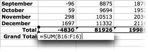
Figure 12-17. The Rangefinder highlights each cell that’s included in the formula you’re currently typing. Furthermore, the color of the outline around the cells matches the typed cell reference.
Formulas do math on values. A value is any number, date, time, text, or cell address that you feed into a formula. The math depends on the operators in the formula—symbols like + for addition,–for subtraction, / for division, * for multiplication, and so on.
Tip
Your formulas don’t have to remain invisible until clicked. To reveal formulas on a given sheet, press Control-` (the key in the upper-left corner of most keyboards). This command toggles the spreadsheet cells so that they show formulas instead of results. (Excel widens your columns considerably, as necessary, to show the formulas.) To return things to the way they were, press Control-` again.
Consider that keystroke a shortcut for the official way to bring formulas into view: Excel → Preferences → View panel. Under Window options, click Formulas; click OK. Repeat the whole procedure to restore the results-only view. Aren’t you glad you’ve now memorized the Control-` shortcut?
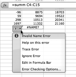
If you make a mistake when you’re typing in a formula, Excel’s error-checking buttons attempt to return you to the straight and narrow. For example, if you type =suum E3:E6, Excel displays “#NAME?” in the cell. Click the cell to display the error-checking button, as shown in Figure 12-18. Clicking the tiny arrow on the right of the button displays several options and bits of information, like the following:
Error Name. The name of the error heads the list. Fortunately, it’s a descriptive name of the error, like Invalid Name Error.
Help on this Error. Click here to view the Excel Help screen on this particular error. This information may help you understand where you went wrong.
Figure 12-18. If you choose to edit the formula in the Formula bar, the alleged formula becomes active in the Formula bar. There you can edit it, and with any luck fix the problem. Note that when presented in the Formula bar, the formula’s cell references are color coded to indicate which color-coded cell they apply to.
Trace Error. Draws lines to the cells that might be causing the errors. Examine the cells in question to determine what you might have done incorrectly.
Ignore Error. The computing equivalent of saying “never mind.” Choosing this item tells Excel to leave the formula as you entered it. (Excel obeys you, but let’s hope you know more than Excel does—there’s no guarantee that the formula will work.)
Edit in Formula Bar. This option lets you edit the formula in the Formula bar as described in Figure 12-18.
Error Checking Options. Opens the Excel → Preferences → Error Checking tab. Here you can turn error checking on and off, and tell Excel which kinds of errors to look for, like empty or missing cells in formulas.
To enter a simple formula that you know well, just double-click the cell and start typing (or click the Edit box in the Formula bar, shown in Figure 12-18, and typed there). The cursor appears simultaneously in the cell and in the Edit box, signaling that Excel awaits your next move.
Your next move is to type an equal sign (=), since every formula starts that way. Then type the rest of the formula using values and operators. When you want to incorporate a reference to a particular cell in your formula, you don’t actually have to type out B12 or whatever—just click the cell in question. Similarly, to insert a range of cells, just drag through them.
Tip
If you mess up while entering a formula and want to start fresh, click the Cancel button at the right end of the Formula bar. (It looks like an X.)
To complete a formula press Enter, Return, Tab, or an arrow key—your choice.
When you tire of typing formulas from scratch (or, let’s be honest, when you can’t figure out what to type), you can let Excel do the brainwork by using functions. Functions are just predefined formulas. For example, the SUM function adds a range of specified values [ =SUM(B3:B7) ] so you don’t have to type the plus sign between each one [ =B3+B4+B5+B6+B7 ]. Excel 2008 adds Formula AutoComplete and the Formula Builder to help you find and enter functions properly. In addition, Excel Help is a veritable Function University with detailed information and examples for all of its functions.
Screen tips (Figure 12-19) for function help are a real boon to spread-sheeting neophytes and dataheads alike. As you start to type a function into a cell, AutoComplete pops up a list of function names matching what you’ve typed so far. Click one to add it to the cell. Then a screen tip displays the syntax of the function in a pale yellow box just below where you’re typing. Not only does the screen tip show you how to correctly type the function it believes you have in mind, but you can also use the screen tip in other ways. For example, you can drag the screen tip to reposition it (to get a better look at your worksheet), click a piece of the tip to select it, or click the function to open up its Help topic in a separate window.
You don’t need access to Microsoft’s reams of focus-group studies to realize that the most commonly used spreadsheet function is adding things up. That’s why Excel comes equipped with a toolbar button that does nothing but add up the values in the column directly above, or the row to the left of, the active cell, as Figure 12-20 shows. (The tutorial that resumes on “Tutorial 2: Yearly Totals” also shows why AutoSum is one of the most important buttons in Excel.)
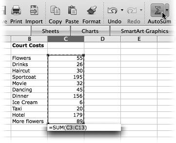
Figure 12-20. The powerful AutoSum button on the Standard toolbar (upper right) is the key to quickly adding a row or column. A click of the button puts a SUM function in the selected cell, which assumes that you want to add up the cells above it. Note that it doesn’t write out C3+C4+C5+C6+C7+C8+C9, and so on; it sets up a range of numbers using the shorthand notation C3:C13. When you press Return, you see only the result, not the formula.
The flippy triangle to the right of the AutoSum button reveals a menu with a few other extremely common options, such as the following:
Average. Calculates the average (the arithmetic mean) of the numbers in the column above the active cell. For example, if the column of numbers represents your Web site revenues for each month then using this function gives you your average monthly income.
Count Numbers. Tells you how many cells in a selected cell range contain numbers.
Max and Min. Shows the highest or lowest value of any of the numbers referred to in the function.
More Functions.When you choose this command, the Formula Builder appears, described shortly.
Tip
After you click the AutoSum button (or use one of its pop-up menu commands), Excel assumes that you intend to compute using the numbers in the cells just above or to the left of the highlighted cell. It indicates, with a moving border, which cells it intends to include in its calculation.
But if it guesses wrong, simply grab your mouse and adjust the selection rectangle by one of its corner handles or just drag through the numbers you do want computed. Excel redraws its border and updates its formula. Press Enter to complete the formula.
Whipping up the sum or average of some cells is only the beginning. Excel is also capable of performing the kinds of advanced number crunching that can calculate interest rates, find the cosine of an arc, find the inverse of the one-tailed probability of the chi-squared distribution, and so on. It’s safe to say that no one has all of these functions memorized.
Fortunately, you don’t have to remember how to write each function; save that brainpower for the Sunday Times crossword. Instead, you can use Excel’s new Formula Builder to look up the exact function that you need. To call up the Formula Builder, click the fx button on the formula bar, choose View → Formula Builder, or click the Toolbox button on the Standard toolbar and then click the fx button .
The new Formula Builder takes the place of Excel 2004’s Paste Function dialog box and greatly simplifies finding and inserting functions. The top of the Formula Builder displays a search field (see Figure 12-21) where you can type any bit of information relating to the function you’re looking for. You can type cosine, for example, and the Formula Builder displays in its main panel the six functions, which somehow relate to cosine. Click any of the functions to read a brief description and the syntax for that function. Double-clicking the function does two things: it inserts the function in the active cell of your spreadsheet and opens the Arguments pane of the Format Builder where it displays the arguments (if any) it’s extracted from your spreadsheet, and at the bottom of the window displays the result.
Just like when you use the AutoSum button, if Excel guesses wrong and highlights the wrong cells in your spreadsheet, either readjust the selection rectangle or click the appropriate cells. Press Return to enter the function into your spreadsheet.
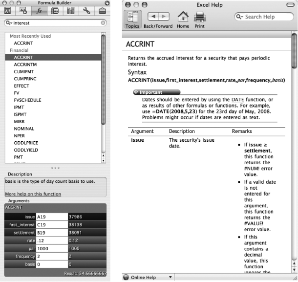
Figure 12-21. The Formula Builder (left) is Excel 2008’s welcome new addition to the Toolbox. You can focus your hunt for the correct one from among the hundreds offered by using the search field at the top of the window. Double-click a function to open the arguments pane, where you can fill in the arguments by clicking cells and making entries directly in this window. When complete, the Formula Builder displays the result at the bottom. To learn more about any specific function, for more assistance with the arguments, or to view sample examples, click “More help on this function” to summon the Excel Help window for that function (right).
What with all the operators, parentheses, cell addresses, functions and such—all of which have to be entered in exactly the correct order—assembling a formula can be a painstaking business. The new formula builder eases much of that pain, but you can choose another approach to formula creation: Excel’s built-in calculator.
Choose Tools → Calculator to summon this virtual pocket pal which features a lot of the standard buttons that you might find on a pocket calculator, plus parentheses buttons, an IF button (to insert an IF statement), and a SUM button (to insert a SUM function). As shown in Figure 12-22, the Calculator window also has three fields: a large one up top that displays the current formula (and also lets you type your own formula, if you’re so inclined) and two smaller ones below it, which show the answer to the formula and the formula’s destination cell.
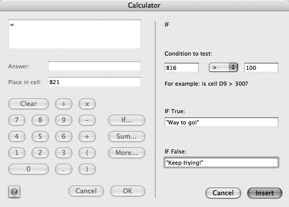
Figure 12-22. The Calculator lets you build a formula with just a few button clicks—in this case, an IF statement that presents different messages depending on the value of B16. Once you’ve perfected the formula, click OK to insert it into the active cell.
To create a formula, click the calculator’s buttons as you would on a real calculator. If you prefer clacking on your keyboard, you can also enter the numbers that way. As you build your formula with the various calculator buttons, the formula shows up in the top window, and the result of the calculation shows up in the Answer field.
Once you’ve built your formula, click OK to paste it into the spreadsheet. (And show it off to your friends who use Excel for Windows, as they don’t yet have a calculator.)
If you want to access other functions (besides the IF and SUM functions), click More to bid the calculator adieu and return to the more knowledgeable Formula Builder.
Tip
If you need a little help with a balky formula that you’ve already entered (perhaps you haven’t gotten its syntax just right), select the cell and open the Formula Builder. It helpfully displays its Arguments pane for the formula in question, so you can see the error of your ways—or the error of your formula, at least.
As you no doubt recall from your basic algebra class, you get different answers to an equation depending on how its elements are ordered. So it’s important for you, the purveyor of fine Excel formulas, to understand the order in which Excel makes its calculations.
If a formula is spitting out results that don’t jibe with what you think ought to be the answer, consult the following table. Excel calculates the operations at the top of the table first, working its way down until it hits bottom. For example, Excel computes cell references before it tackles multiplication, and it does multiplication before it works on a “less than” operation.
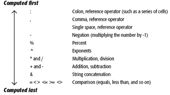
For example, Excel’s answer to =2+3*4 is not 20. It’s 14, because Excel performs multiplication and division within the formula before doing addition and subtraction.
You can exercise some control over the processing order by using parentheses. Excel calculates expressions within ( ) symbols before bringing the parenthetical items together for calculation. So in the above example, =(2+3)*4 returns 20. Or, the formula =C12*(C3-C6) subtracts the value in C6 from the value in C3 and multiplies the result by the value in C12. Without the parentheses, the formula would read =C12*C3-C6, and Excel would multiply C12 by C3 and then subtract C6—a different formula entirely.
Suppose you’ve entered a few numbers into a spreadsheet, as described in the tutorial earlier in this chapter. Finally it’s time to put these numbers to work. Open the document shown in Figure 12-16.
Now that it has some data to work with, Excel can do a little work. Start with one of the most common spreadsheet calculations: totaling a column of numbers. First create a row for totals.
Click cell A17 (leaving a blank row beneath the month list). Type Total.
This row will soon contain totals for each year column.
Click cell B17, in the Total row for 2004. Click the AutoSum button on the Standard toolbar.
In cell B17, Excel automatically proposes a formula for totaling the column of numbers. (It’s =SUM(B3:B16), meaning “add up the cells from B3 through B16.”) The moving border shows that Excel is prepared to add up all of the numbers in this column—including the year label 2004! Clearly, that’s not what you want, so don’t press Enter yet.
Drag through the numbers you do want added: from cell B4 down to B15. Then press Return.
Excel adds up the column.
Now comes the real magic of spreadsheeting: If one of the numbers in the column changes, the total changes automatically. Try it.
Click one of the numbers in column B, type a much bigger number, and then press Return.
Excel instantly updates 2004’s total to reflect the change.
Tip
The AutoSum feature doesn’t have to add up numbers above the selected cell; it can also add up a row of cells. In fact, you can even click the AutoSum button and then drag through a block of cells to make Excel add up all of those numbers.
You could continue selecting the Total cells for each year and using AutoSum to create your totals. Instead, you can avoid repetition by using the Fill command described earlier in this chapter. You can tell Excel to create a calculation similar to the 2004 total for the rest of the columns in the spreadsheet.
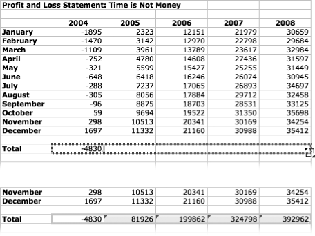
Click the cell containing the 2004 total (B17) and drag the selection’s Fill handle (see Using the Fill handle) to the right, all the way over to the 2008 column (F17).
As you drag, Excel highlights the range of cells for column totals, and when you release your mouse, it fills those cells with column totals as shown in Figure 12-23.
You could’ve accomplished the same thing by first just selecting the range of cells and then choosing Edit → Fill → Right—but why would you want to?
Either way, Excel copies the contents of the first cell and pastes it into every other cell in the selection. In this example, the first cell contains a formula, not just a total you typed yourself. But, instead of pasting the exact same formula, which would place the 2004 total into each column, Excel understands that you want to total each column, and therefore enters the appropriate formula in each cell of your selection. The result is yearly totals calculated right across the page.
Finally, to make the yearly totals in the tutorial example more meaningful—and see just how much money you actually made—calculate an overall total for the spreadsheet.
Click cell A19 and type Grand Total and then press Tab.
Excel moves the active cell to B19.
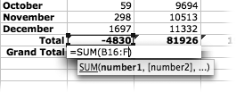
To calculate a lifetime total for the spreadsheet, you need to tell Excel to add together all the yearly totals.
Click the AutoSum button on the Standard toolbar.
In this case, the cells you want to add aren’t lined up with the Grand Total cell, so the AutoSum button doesn’t work quite right; it proposes totaling the column of numbers above it.
Drag across the yearly totals (from B17 through F17).
As you drag across the cells, Excel inserts the cell range within the formula and outlines the range of cells. In this example, the function now reads, =SUM(B17:F17)—in other words, “add up the contents of the cells B17 through F17, and display the result.”
Press Return (or Enter).
Excel performs the calculation and displays the result in cell B19, the grand total for the rags to riches story of an Internet marketer.
Once your spreadsheet grows beyond the confines of your screen, you may find it difficult to find your way back to areas within it that you work on the most frequently. By designating a cell or group of cells as a named range, you can quickly jump to a certain spot without having to scroll around for it. You can use named cells as a quick way to navigate a large spreadsheet. Once you’ve created a named range, click the Name pop-up menu in the Formula bar and choose it from the list. Excel instantly transports you to the correct corner of your spreadsheet, where you’ll find the named range selected and waiting for you.
As you create formulas, you may find yourself referring over and over to the same cell or range of cells. For example, in the profit and loss spreadsheet (Figure 12-23), you may need to refer to the 2008 Total in several other formulas. So that you don’t have to repeatedly type the cell address or click to select the cell, Excel lets you give a cell, or range of cells, a name. After doing so, you can write a formula in the form of, for example, =Total2008-Taxes (instead of =B17-F27). Or, you may find yourself doing the same operation on the same range of cells over and over, for example, totaling or averaging your monthly expenses. By designating a monthly expense totals as a named range, you can create surprisingly readable formulas that look like =SUM(Expenses) or =AVERAGE(Expenses).
To create a named cell or range, simply select the cell or range, enter a name for it in the Formula bar’s Name box, and press Return (or choose Insert → Name → Define) as shown in Figure 12-24.
Note
Named ranges take one-word names only: Excel doesn’t accept spaces or hyphens. And, as you’d expect, no two names can be the same on the same worksheet: Excel considers upper- and lowercase characters to be the same, so profit is the same as PROFIT. Additionally, the first character of a name has to be a letter (or an underscore); names can’t contain punctuation marks (except periods) or operators (+, =, and so on); and they can’t take the form of a cell reference (such as B5) or a function (such as SUM()).
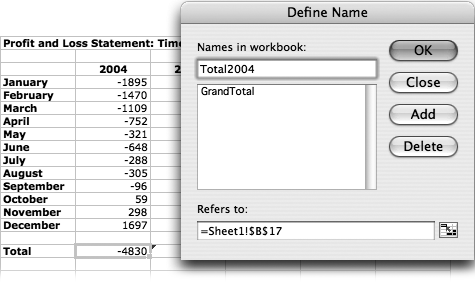
Figure 12-24. To name a cell or range of cells, select it, enter a name for it in the Formula bar’s Name box, and press Return. From now on, you can use the Name box pop-up menu to jump directly to that point in your spreadsheet.
From now on, the cell’s or range’s name appears in the Formula bar’s Name pop-up menu. The next time you want to go to that cell or range or use it in a formula, you need only click that pop-up menu and select it from the list. In addition, Excel displays the name instead of the cell address whenever you create a formula that refers to a named cell or range.
If you need to change or remove a name, choose Insert → Names → Define to display the Define Names dialog box. From there, you’ll find it easy to delete, create, or edit names.
When you create a formula by typing the addresses of cells or by clicking a cell, you’ve created a cell reference. However, rather than always meaning B12, for example, Excel generally considers cell references in a relative way—it thinks of another cell in the spreadsheet as “three rows above and two columns to the left of this cell,” for example (see Figure 12-25). In other words, it remembers those cell coordinates by their position relative to the selected cell.
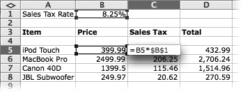
Figure 12-25. The formula in cell C5 calculates the sales tax for the item priced in B5. The sales tax rate is stored in B1. Thus, the formula in C5 multiplies the price (B5) by an absolute reference to the sales tax rate (expressed $B$1). When you copy this formula, it always refers to the fixed cell B1.
Relative cell references also make formulas portable: When you paste a formula that adds up the two cells above it into a different spot, the pasted cell adds up the two cells above it (in its new location).
The yearly totals in Figure 12-23 show how this works. When you “filled” the Total formula across to the other cells, Excel pasted relative cell references into all those cells that say, in effect, “Display the total of the numbers in the cells above this cell.” This way, each column’s subtotal applies to the figures in that column. (If Excel instead pasted absolute references, then all the cells in the subtotal row would show the sum of the first-year column.)
Absolute references, on the other hand, refer to a specific cell, no matter where the formula appears in the spreadsheet. They can be useful when you need to refer to a particular cell in the spreadsheet—the one containing the sales tax rate, for example—for a formula that repeats over several columns. Figure 12-25 gives an example.
You designate an absolute cell reference by including a $ in front of the column and/or row reference. (For the first time in its life, the $ symbol has nothing to do with money.) For example, $A$7 is an absolute reference for cell A7.
You can also create a mixed reference in order to lock the reference to either the row or column—for example, G$8, in which the column reference is relative and the row is absolute. You might use this unusual arrangement when, for example, your column A contains discount rates for the customers whose names appear in column B. In writing the formula for a customer’s final price (in column D, for example), you’d use a relative reference to a row number (different for every customer), but an absolute reference to the column (always A).
Tip
There’s a handy shortcut that can save you some hand-eye coordination when you want to turn an absolute cell reference into a relative one, or vice versa. First, select the cell that contains the formula. In the Formula bar, highlight only the cell name you’d like to change. Then press ⌘-T. This keystroke makes the highlighted cell name cycle through different stages of absoluteness—for example, it changes the cell reference B4 first to $B$4, then to B$4, then to $B4, and so on.