Chapter 12 covers the fundamentals of formulas—entering them manually, using the Formula Builder, and so on. The following section dives deeper into the heart of Excel’s mathematical power—its formulas.
Note
There’s a difference between formulas and functions. A formula is a calculation that uses an arithmetic operator (such as =A1+A2+A3+A4+A5), while a function is a canned formula that saves you the work of creating a formula yourself (such as =SUM(A1:A5)).
Because there’s no difference in how you use them, this chapter uses the terms interchangeably.
A nested formula is a formula that’s used as an argument (see the box on Looking up functions with the Formula Builder) to another formula. For example, in the formula =ABS(SUM(A1:A3)), the formula SUM(A1:A3) is nested within an absolute-value formula. When interpreting this formula, Excel first adds the contents of cells A1 through A3, and then finds the absolute value of that result—that’s the number you’ll see in the cell.
Nested formulas keep you from having to use other cells as placeholders; they’re also essential for writing compact formulas. In some cases (such as with the logical IF function), nesting lets you add real sophistication to your Excel spreadsheets by having Excel make decisions based on formula results.
The Formula Builder is a quick way of building powerful mathematical models in your spreadsheets. When activated, the Formula Builder shows every imaginable aspect of a formula: the value of the cells used in it, a description of what the formula does, a description of the arguments used in the formula, and the result of the formula.
To use the Formula Builder, click the Toolbox button in the toolbar and click the Toolbox’s fx tab. When the Formula Builder pops up (Figure 14-7), it shows one of two things:
If the currently active cell doesn’t contain a function, the bottom of the Formula Builder says “To begin, double-click a function in the list.” Use the Search field or scroll through the Formula Builder’s long, long list to find your function.
If the currently active cell contains a function, or if you type a function into your formula, the Formula Builder opens fully and tries to help you with the function.
Once the Formula Builder appears, you can use it to construct your formula. It provides a text box for each function parameter. Typing the parameter in the text box effectively inserts it into its proper place in the formula. You can also click cells or drag through cells in the spreadsheet to insert the cell reference or range in the Formula Builder.
As you fill out the formula in the Formula Builder, the formula’s result appears in the bottom of the palette as well as in the active cell. When you’re done creating the formula in the Formula Palette, press Return to enter it in the cell.
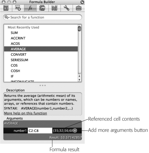
Figure 14-7. Excel’s Formula Builder conveniently presents an amazing amount of information about a selected cell’s formula. It’s especially helpful for times when you know something about the formula that you’re entering, but you need a little help with the details. The Formula Builder not only shows the result of the formula but also lists the arguments and the referenced cell contents. It gives a short description of the function and shows its syntax. Click “More help on this function” to open the functions page in Excel Help for a more detailed description and further examples. You can modify your function by editing directly in this window; click the plus-sign button to add more arguments.
Although the Formula Builder might seem like overkill when it comes to simple formulas (such as a SUM), it’s a big help when you’re dealing with more complex formulas. It outlines the parameters that the formula is expecting and gives you places to plug in those parameters. The rangefinder feature (Formula Fundamentals) also makes it easier to track your calculations. (The rangefinder highlights each cell cited in the calculation with the same color used to denote the cell in the calculation. It’s a sharp way to keep track of what you’re doing, and which cells you’re doing it with.)
If you create a formula that, directly or indirectly, refers to the cell containing it, beware of the circular reference. This is the spreadsheet version of a Mexican standoff: The formula in each cell depends on the other, so neither formula can make the first move.
Suppose, for example, you type the formula =SUM(A1:A6) into cell A1. This formula asks Excel to add cells A1 through A6 and put the result in cell A1—but since A1 is included in the range of cells for Excel to add, things quickly get confusing. To make matters worse, a few specialized formulas actually require that you use formulas with circular references. Now, imagine how difficult it can be to disentangle a circular reference that’s inside a nested formula that refers to formulas in other cells—it’s enough to make your teeth hurt. Fortunately, Excel can help.
For example, when you enter a formula containing a circular reference, Excel immediately interrupts your work with a dialog box that explains what’s happening. You may enter a formula that doesn’t itself contain a circular reference, but instead completes a circular reference involving a group of cells. Or the formulas in two different cells might refer to each other in a circular fashion, as shown in Figure 14-8.
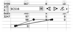
Figure 14-8. Double-click the tracer arrow to jump to the next cell involved in the circular reference, or click the buttons on the toolbar. With these tools, Excel reveals the various cells involved in the circular reference; eventually, you should be able to untangle the problem.
To leave the formula as is, click Cancel. For help, click OK, which brings up a Microsoft Office Help window loaded with directions and the Circular Reference toolbar. (Excel also overlays circles and tracer arrows on the cells of your spreadsheet.)
On the other hand, certain functions (mostly scientific and engineering) need circular references to work properly. For example, if you’re doing a bit of goal-seeking (Goal seek), you can use circular references to plug numbers into a formula until the formula is equal to a set value.
In these cases, Excel has to calculate formulas with circular references repeatedly, because it uses the results of a first set of calculations as the basis for a second calculation. Each such cycle is known as an iteration. For example, suppose you want to figure out what value, when plugged into a formula, will produce a result of 125. If your first guess of 10 gives you a result of 137 when plugged into the formula, a circular reference can use that result to adjust your guess (say, reducing it to 9.5), then make a second pass at evaluating the formula. This second pass is a second iteration. If 9.5 doesn’t do the trick, Excel can make a third iteration to get even closer, and so on, until it reaches a level of accuracy that’s close enough.
To turn iteration on (and set some of its parameters), choose Excel → Preferences; click Calculation. In the Calculation panel, turn on Limit Iteration, and change the number of iterations and, if you like, a maximum change value. Excel automatically stops after 100 iterations, or when the difference between iterations is smaller than 0.001. If you make the maximum number of iterations larger or the maximum change between iterations smaller, Excel can produce more accurate results. Accordingly, it also needs more time to calculate those results.
Formulas aren’t necessarily confined to data in their own “home” worksheet; you can link them to cells in other worksheets in the same workbook, or even to cells in other Excel documents. That’s a handy feature when, for example, you want to run an analysis on a budget worksheet with your own set of Excel tools, but you don’t want to re-enter the data in your workbook or alter the original workbook.
To link a formula to another sheet in the same workbook, start typing your formula as you normally would. When you reach the part of the formula where you want to refer to the cells in another worksheet, click the sheet’s tab to bring it to the front. Then select the cells that you want to appear in the formula, just as you normally would when building a formula. When you finish clicking or dragging through cells, press Enter and Excel instantly returns you to the sheet where you were building the formula. In the cell, you’ll find a special notation that indicates a reference to a cell on another sheet. For example, if a formula on Sheet 3 takes the sum of G1 through G6 on Sheet 1, the formula looks like this: =SUM(Sheet1!G1:G6).
To link a formula in Document A to cells in another workbook (Document B), the process is almost identical. Start typing the formula in Document A. Then, when it’s time to specify the cells to be used in the formula, open Document B. Select the cells you want to use by clicking or dragging; when you press Enter, they appear in the formula. Excel returns you to the original document, where you’ll see the Document B cells written out in a path notation (see Figure 14-9).
Once you’ve set up such a cell reference, Excel automatically updates Document A each time you open it with Document B already open. And if Document B is closed, Excel asks if you want to update the data. If you say yes, Excel looks into Document B and grabs whatever data it needs. If somebody has changed Document B since the last time Document A was opened, Excel recalculates the worksheet based on the new numbers.
Figure 14-9. External cell references display the path to the worksheet of the external spreadsheet between single quotation marks in the formula bar. If you move the file or rename any volumes or folders along the path, you’ll break the link. You can manually update the external reference in the formula bar, but it’s often easier to just double-click the cell, press Return, navigate back to the external document, and let Excel update the reference. (And you won’t risk a path-breaking typo.)
Tip
If you want Document A updated automatically whenever you open it (and don’t want to be interrupted with Excel’s request to do so), choose Excel → Preferences, click Edit, and then turn off “Ask to update automatic links.” Excel now automatically updates the link with the data from the last saved version of Document B.
Every now and then, you’ll find a formula whose cell references are amiss. If the formula references another formula, tracing down the source of your problems can be a real pain. Excel’s Auditing tools can help you access the root of formula errors by showing you the cells that a given formula references and the formulas that reference a given cell. Brightly colored tracer arrows (these won’t appear in an Excel workbook saved as an HTML file) appear between cells to indicate how they all relate to each other.
The key to correcting formula errors is the Tools → Auditing menu item, which has five submenu choices:
Trace Precedents draws arrows from the currently selected cell to any cells that provide values for its formula.
Trace Dependents draws arrows from the currently selected cell, showing which other formulas refer to it.
Trace Error draws an arrow from an active cell containing a “broken” formula to the cell or cells that caused the error.
Show Auditing Toolbar hides or shows the Auditing Toolbar. This toolbar’s buttons turn on (and off) the kinds of arrows described in the previous paragraphs, all in an effort to help you trace how formulas and cells relate with each other. It also contains buttons for attaching comments, for circling invalid data, and for removing those circles.