When it comes to spreadsheets, the term formatting covers a lot of ground. It refers to the size of the cell, how its borders look, what color fills it, as well as how the contents of the cell are formatted (with or without dollar signs or decimal points, for example)—anything that affects how the cell looks.
Excel offers two ways to add formatting to your spreadsheet: by using Excel’s automatic formatting capabilities or by doing the work yourself. Odds are, you’ll be using both methods.
If you’re not interested in hand-formatting your spreadsheets—or you just don’t have the time—Excel’s AutoFormat tool is a quick way to apply formatting to your sheets. It instructs Excel to study the layout and contents of your spreadsheet and then apply colors, shading, font styles, and other formatting attributes to make the sheet look professional.
Note
AutoFormat is best suited for fairly boring layouts: column headings across the top, row labels at the left side, totals at the bottom, and so on. If your spreadsheet uses a more creative layout, AutoFormat may make quirky design choices.
To use the AutoFormat feature, select the cells you want formatted, and then choose Format → AutoFormat. The AutoFormat dialog box appears, complete with a list of formats on the left (see Figure 13-1). By clicking each one in turn, you’ll see (in the center of the dialog box) that each one is actually a predesigned formatting scheme for a table-like makeover of the selected cells.
On the right is a button labeled Options, which lets you control the formatting elements that will be applied to the selected cells.
Once you’ve selected an AutoFormat option (and made any tweaks to the applied formats), click OK. Excel goes to work on the selected cells (see Figure 13-1). If you don’t care for the results, you can always undo them with a quick ⌘-Z.
Another way to quickly apply formatting to a group of cells is the Format Painter. Suppose you’ve painstakingly applied formatting—colors, cell borders, fonts, text alignment, and the like—to a certain patch of cells. Using the Format Painter, you can copy the formatting to any other cells—in the same or a different spreadsheet.
To start, select the cell(s) that you want to use as an example of good formatting. Then click the Format button (the little paintbrush) on the Standard toolbar.
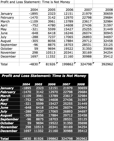
Figure 13-1. The AutoFormat dialog box is an expeditious way to make your spreadsheets more readable—and more attractive. You can transform the stock Excel appearance (top) to an eye-catching and more comprehensible presentation (bottom) with two quick clicks. Each scheme may include font selections, shadings for table rows, background patterns, and so on.
Now, as you move the cursor over the spreadsheet it changes to look like a + sign and a paintbrush.
Next, drag the cursor over the cells (or click a single cell) you’d like to change to match the first group. Excel applies the formatting—borders, shading, font settings, and the like—to the new cells (Figure 13-2).
If the AutoFormat feature is a bit too canned for your purposes, you can always format the look of your spreadsheet manually. When formatting cells manually, it’s helpful to divide the task up into two concepts—formatting the cells themselves (borders and backgrounds), and formatting the contentsof those cells (what you’ve typed).
When you open an Excel worksheet, all the cells are the same size. Specifically, they’re 1.04 inches wide (the factory-set width of an Excel column) and 0.18 inches tall (the height of an Excel row). The good news is that there are several ways to set a cell’s height and width. Here’s a rundown:
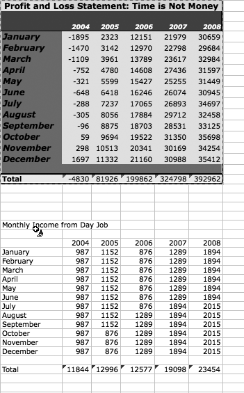
Figure 13-2. The Format Painter can take everything but the data from the cells on the top, and apply it to the cells on the bottom.
Note
If you use the Metric system, you can change to centimeters or millimeters on the Excel → Preferences → General tab. Choose from the “Measurement units” pop-up menu. Unfortunately, 4.59 millimeters is just as hard to remember as 0.18 inches.
Dragging the borders. Obviously, you can’t enlarge a single cell without enlarging its entire row or column; Excel has this funny way of insisting that your cells remain aligned with each other. Therefore, you can’t resize a single cell independently—you can only enlarge its entire row or column.
To adjust the width of a column, drag the divider line that separates its column heading from the one to its right, as shown in Figure 13-3; to change the height of a row, drag the divider line between its row and the one below it. In either case, the trick is to drag in the row numbers or column letters. Your cursor will look like a bar between two arrows if you drag in the right place.
Note
Excel adjusts row heights automatically if you enlarge the font or wrap your text by turning on the Wrap text control in Format → Cells → Alignment (unless you’ve set the height manually, as described above).
Figure 13-3. Changing the width (top) of a column or height of a row is as simple as dragging its border in the column letters or row numbers. A small yellow box pops up as you drag, continually updating the exact size of the column or row. When you let go of the mouse, the column or row assumes its new size, and the rest of the spreadsheet moves to accommodate it. If you select multiple columns or rows, dragging a border changes all of the selected columns or rows—a lovely way to keep consistent spacing.
Menu commands. For more exact control over height and width adjustments, choose Format → Row → Height, or Format → Column → Width. Either command pops up a dialog box where you can enter the row height or column width by typing numbers on your keyboard.
Autosizing. For the tidiest spreadsheet possible, highlight some cells and then choose Format → Row → AutoFit, or Format → Column → AutoFit Selection. Excel readjusts the selected columns or rows so they’re exactly as wide and tall as necessary to contain their contents, but no larger. That is, each column expands or shrinks just enough to fit its longest entry.

Tip
You don’t have to use the AutoFit command to perform this kind of tidy adjustment. You can also, at any time, make an individual row or column precisely as large as necessary by double-clicking the divider line between the row numbers or the column letters. (The column to the left of your double-click, or the row above your double-click, gets resized.) When using this method, there’s no need to highlight anything first.
There are any number of reasons why you may want to hide or show certain columns or rows in your spreadsheet. Maybe the numbers in a particular column are used in calculations elsewhere in the spreadsheet, but you don’t need them taking up screen space. Maybe you want to preserve several previous years’ worth of data, but don’t want to scroll through them. Or maybe the IRS is coming for a visit.
In any case, it’s easy enough to hide certain rows or columns. Start by highlighting the rows or columns in question. (Remember: To highlight an entire row, click its gray row number; to highlight several consecutive rows, drag vertically through the row numbers; to highlight nonadjacent rows, ⌘-click their row numbers. To highlight certain columns, use the gray column letters at the top of the spreadsheet in the same way.)
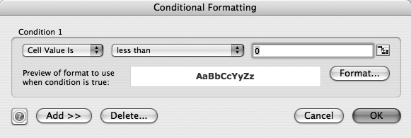
Figure 13-4. Choose Format → Conditional Formatting to make cells style their contents according to the conditions you set in this dialog box. Let Excel tell you when your finances are “in the red” by formatting any negative numbers with that eye-catching color. Use the pop-up menus in the first line to set the condition and then click the Format button to tell Excel how to format the cell when that condition is met.
Next, choose Format → Row → Hide, or Format → Column → Hide. That’s all there is to it: The column or row disappears completely, leaving a gap in the numbering or letter sequence at the left or top edge of the spreadsheet. The row numbers or column letters surrounding the hidden area turn blue.
Making them reappear is a bit trickier, since you can’t exactly highlight an invisible row or column. To perform this minor miracle, use the blue-colored row numbers or column headers as clues. Select cells on either side of the hidden row or column. Then choose Format → Row → Unhide, or Format → Column → Unhide.
Alternatively, you can also select a hidden cell (such as B5) by typing its address in the Name box on the Formula bar, and then choosing Format → Row → Unhide, or Format → Column → Unhide.
The light gray lines that form the graph-paper grid of an Excel spreadsheet are an optical illusion. They exist only to help you understand where one column or row ends and the next begins, but they don’t print (unless you want them to; see Sheet tab).
If you’d like to add solid, printable borders to certain rows, columns, or cells, Excel offers three different methods: the old, but most versatile Format Cells dialog box, the “Borders and Shading” section of the Formatting Palette, and the very similar Border Drawing toolbar. All techniques let you control how lines are added to the cell’s edges, but only the Formatting Palette and the toolbar let you change borders and shading without first opening a dialog box to make the changes.
To add cell borders using the time-honored Format Cells command, highlight some cells and then choose Format → Cells (or press ⌘ -1). The Format Cells dialog box appears; now click the Border tab to show the border controls. In this tab, you’ll see three sections: Presets, Border, and Line (see Figure 13-5).
If you don’t want to use the default line style and color, choose new ones in the Line section.
Excel loads your cursor with your desired style and color.
Figure 13-5. Click directly in the preview area inside the Border section to place borders where you want them. First, select the style and color of line on the right side, and then click in the preview area to place the line. Or if you’re feeling more button-oriented, use the eight buttons around the left and bottom edges of the preview area to draw your horizontal and vertical borders, and the oft-overlooked diagonals.
To create a border around the outside of your selection, click the Outline preset button; to create borders for the divisions inside your selection, click the Inside button; and click both buttons for borders inside and around your selection.
As you click the buttons, Excel displays a preview of your work in the Border section. If you change your mind, click None to remove the option.
If the Outline and Inside presets aren’t what you have in mind, apply custom borders. Click directly between the guides in the preview pane to add or delete individual borderlines, or use the buttons that surround the preview.
To change a line style, reload the cursor with a new style from the Line section and then click the borders in the preview area you wish to change.
If you mess up, click None in the Presets area and start again.
Once the borders look the way you’d like, click OK.
Excel applies the borders to the selection in your spreadsheet.

To use Excel’s Formatting Palette to draw borders, select the cells to work with, and then open the “Borders and Shading” portion of the palette by clicking the “Borders and Shading” Title Bar.
In this section of the palette, you’ll see six controls that help you box in your cells and apply colors and patterns (Figure 13-6).
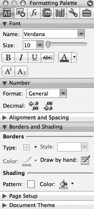
Figure 13-6. The Formatting Palette’s “Borders and Shading” section makes adding borders to your spreadsheet painless. Click the flippy triangle to the left of “Borders and Shading (or anywhere on that bar) to show or hide the controls. If you don’t see the Formatting Palette, choose its name from the View menu, or click the Toolbox button in the toolbar and then click its Formatting Palette button.
Here’s what each control does:
Type. The button itself indicates the kind of border you’ve already applied to the selected cells; if you haven’t applied a border, the icon on the button is a faint, dotted-line square. In any case, click it to open a pop-out palette of 18 different border styles, covering most conceivable border needs. The first 12 borders are standard fare, mostly outlines and single lines. The last six styles show more variety; some put borders on two sides of a selection or include thicker borders on one side. (If you point to one of these border styles without clicking, a yellow pop-up screen tip gives a plain-English description of its function.)
This pop-up palette should be your first stop. Some of the other palettes described here aren’t even available until you’ve first selected a border type.
Style. Choose a line style, such as dotted lines or thick lines.
Color. This button lets you choose from one of 40 preset line colors. Note that you can also leave the line color set to Automatic (which usually means black) if you choose.
Tip
If the idea of 40 preset colors puts the artist in you into a huff, calm down—you can mix your own presets. Choose Excel → Preferences → Color, choose one of the presets, and click Modify. Blend a new hue and you’ll find it available anywhere Excel uses color. Even better, if you’ve already used that preset color, Excel changes it to reflect your new choice.
Pattern. Instead of changing the style of line surrounding the selected cells, this button offers patterns with which to fill the selected cells’ backgrounds. (The bottom half of this menu specifies the color that Excel will use to draw the black areas of the displayed patterns.) You’ll probably find that most of the patterns make your cell contents illegible, unless you also select a very light color for the fill. However, both pattern and fill color can be very useful for headings or areas of your spreadsheet that don’t display text. (“Automatic,” by the way, means “no pattern.”)
Fill color. Clicking this button reveals options for 40 preset fill colors for your cell backgrounds. Here again, use this option with caution; unless you also change the text color to a contrasting color, you should use only very light colors for filling the cell backgrounds. (See the previous Tip to create custom colors.)
Draw borders by hand. Clicking Draw by Hand brings up the Border Drawing toolbar, a Lilliputian toolbar with five unlabeled buttons. (Point to each without clicking to reveal its pop-up yellow label.)
The first one, Draw Border, pops up so you can choose between two modes: Draw Border and Draw Border Grid. The Draw Border tool lets you create a border that encloses an otherwise unaffected block of cells just by dragging diagonally in your spreadsheet; the border takes on the line characteristics you’ve specified using the other tools in the toolbar. The Draw Border Grid tool works similarly, except that it doesn’t draw one master rectangle. Instead, it adds borders to every cell within the rectangle that you create by dragging diagonally, “painting” all four walls of every cell inside.
To erase borders from the spreadsheet, click Erase Border and then drag across any unwanted borders (or those painted in by mistake). Press Esc to cancel the eraser cursor. (The middle button, Merge Cells, is described on Merging cells.) The active extremity of the eraser cursor is the very bottom—which appears to sparkle.
Tip
You can tear palettes off the Formatting Palette, which makes for easy access if you need to get to their functions frequently. To do so, click the Font Color button, for example, and then click the double-dotted line at the top of the pop-out. The Font Color palette “tears off” and becomes a window unto itself.
Borders and fills control how cells look whether or not they actually contain anything. Excel also gives you a great deal of control over the appearance of your text—which in spreadsheets is often numbers. The text controls in Excel are divided into three major categories: number formatting, font control, and text alignment.
Number formats in Excel add symbols, such as dollar signs, decimal points, or zeros, to whatever raw numbers you’ve typed. For example, if you apply Currency formatting to a cell containing 35.4, it appears in the spreadsheet as $35.40; if you apply Percentage formatting, it becomes 3540.00%.
What may strike you as odd, especially at first, is that this kind of formatting doesn’t actually change a cell’s contents. If you double-click the aforementioned cell that says $35.40, the trappings of currency disappear instantly, leaving behind only the 35.4 that you originally entered. All number formatting does is add the niceties to your numbers to make them easier to read.
To apply a number format, select the cells on which you want to work your magic, and then select the formatting that you want to apply. Excel comes prepared to format numbers using eleven broad categories of canned formatting. You get at them in any of three ways:
The Format pop-up menu in the Number section of the Formatting Palette (better known as “the easy way”), as shown in Figure 13-7.
The Format Cells dialog box that appears when you choose Format → Cells (or Control-click some cells and choose Format Cells from the shortcut menu).
The old Formatting toolbar (choose View → Toolbars → Formatting). The new Formatting Palette is light-years more flexible, so if you have the screen space for it, you can safely ignore the Formatting toolbar. (Unless you, as a diehard Excel 98 fan, have a raging antipathy toward change, that is.)
Each method gives the same broad categories of formatting; however, options in the Formatting Palette and toolbar are far fewer. Instead, they apply the most popular choice (for example, $ signs when you choose the currency formatting) without asking your opinion. The Format Cells dialog box, on the other hand, gives you more control over each format, along with a helpful preview of the result.
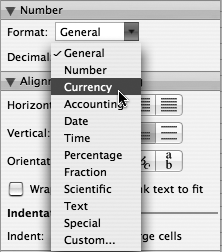
Figure 13-7. The Number section of the Formatting Palette provides quick access to common number formatting options via the Format pop-up menu. It also lets you increase or decrease the number of decimal places shown by clicking the Increase Decimal or Decrease Decimal buttons.
The following descriptions identify which additional controls are available in the Format Cells dialog box:
General. This option means “no formatting.” Whatever you type into cells formatted this way remains exactly as is (see Figure 13-8).
Number. This control formats the contents as a generic number.
Format Cells dialog box extras: You have the option to specify exactly how you want negative numbers to appear, how many decimal places you want to see, and whether or not a comma should appear in the thousands place.
Currency. A specific kind of number format, the Currency format adds dollar signs, commas, decimal points, and two decimal places to numbers entered in the selected cells.
Figure 13-8. Here’s how the 11 different number formats make the number 35396.573 look. Some of the differences are subtle, but important. The contents of Text formatted cells are left-justified, for example, and the Number format lets you specify how many decimal places you want to see. Date and Time formats treat any number you specify as date and time serial numbers—more a convenience for Excel than for you.
Format Cells dialog box extras: You can specify how many decimal places you want to see. You also get a Currency Symbol pop-up menu that lists hundreds of international currency symbols, including the euro. You can also set how Excel should display negative numbers.
Accounting. A specific kind of currency format, the Accounting format adds basic currency formatting—a $ sign, commas in the thousands place, and two decimal places. It also left-aligns the $ sign and encloses negative numbers in parentheses.
Format Cells dialog box extras: You can opt to use a different currency symbol and indicate how many decimal places you’d like to see.
Date. Internally, Excel converts the number in the cell to a date and time serial number (see Times) and then converts it to a readable date format, such as 11/22/2008.
Format Cells dialog box extras: You can specify what date format you want applied, such as 11/22/08, November-08, or 22-Nov-2008.
Time. Once again, Excel converts the number to a special serial number and then formats it in a readable time format, such as 1:32.
Format Cells dialog box extras:The dialog box presents a long list of time-formatting options, some of which include both the time and date.
Percentage. This displays two decimal places for numbers and then adds percent symbols. The number 1.2, for example, becomes 120%.
Format Cells dialog box extras: You can indicate how many decimal places you want to see.
Fraction. This option converts the decimal portion of a number into a fraction. (People who still aren’t used to a stock market statistics represented in decimal form will especially appreciate this one.)
Format Cells dialog box extras: You can choose from one of nine fraction types, some of which round the decimal to the nearest half, quarter, or tenth.
Scientific. The Scientific option converts the number in the cell to scientific notation, such as 3.54E+04 (which means 3.54 times 10 to the fourth power, or 35,400).
Format Cells dialog box extras: You can specify the number of decimal places.
Text. This control treats the entry in the cell as text, even when the entry is a number. (Excel treats existing numbers as numbers, but after you format a cell as Text, numbers are treated as text.) The contents are displayed exactly as you entered them. The most immediate change you’ll discover is that the contents of your cells are left-justified, rather than right-aligned as usual. (No special options are available in the Format Cells dialog box.)
Special. This option formats the numbers in your selected cells as postal Zip codes. If there are fewer than five digits in the number, Excel adds enough zeros to the beginning of the number. If there’s a decimal involved, Excel displays it rounded to the nearest whole number. And if there are more than five digits to the left of the decimal point, Excel leaves the additional numbers alone.
Format Cells dialog box extras: In addition to Zip code format, you can choose from several other canned number patterns: Zip Code + 4, Phone Number, and Social Security Number. In each case, Excel automatically adds parentheses or hyphens as necessary.
Custom. The Custom option brings up the Format Cells dialog box, where you can create your own number formatting, either starting with one of 39 preset formats or writing a format from scratch using a small set of codes. For example, custom formatting can be written to display every number as a fraction of 1000—something not available in the Fraction formatting.

To add or remove decimal places, turning 34 and 125 into 34.00 and 125.00, for example, click the Decimal buttons in the Formatting Palette, as shown in Figure 13-7. Each click on the Increase Decimal button (on the left) adds decimal places; each click on the Decrease Decimal button (on the right) decreases the level of displayed precision by one decimal place.
Excel lets you control the fonts used in its sheets via the Font portion of the Formatting Palette. As always on the Macintosh, highlight what you want to format, and then apply the formatting—in this case using the Formatting Palette.
Of course, you can highlight the cell(s) you want to format using any of the techniques described on Selecting Cells (and Cell Ranges). But when it comes to character formatting, there are additional options; Excel actually lets you apply different fonts and font styles within a single cell (but not for formulae). The trick is to double-click the cell and then use the I-beam cursor to select just the characters in the cell that you want to work with—or select the characters in the Edit box of the Formula bar. As a result, any changes you make in the Formatting Palette affect only the selected characters.
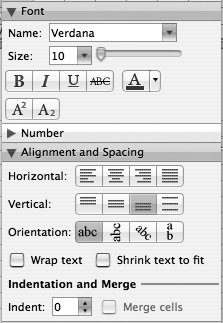
Once you’ve highlighted the cells or text you want to change, open the Fonts section of the Formatting Palette (Figure 13-9) to reveal its four main controls:
The Name pop-up menu lets you apply any active font on your Mac to the highlighted cell(s).
Tip
If your Mac has numerous fonts installed, you may find it faster to specify your desired font by typing its name in the Name field rather than by using the pop-up menu. As you type, Excel’s AutoComplete guesses your intention and produces a pop-up menu for you to choose from. As soon as the correct font name appears, click it (or select it using the up- and down-arrow keys), and press Return.
Figure 13-9. Top: By tweaking the controls in the Font section of the Formatting Palette, you can quickly create your own custom text look. Bottom: The “Alignment and Spacing” section of the Formatting Palette provides precise control over how text fills a cell; it can even be used to join cells together.
The Size pop-up menu lets you choose from commonly used font sizes (9-point, 18-point, and so on). If the size you want isn’t listed, type a number into the Size field and then press Enter or Return. (Excel accommodates only whole- and half-number point sizes. If you type in any other fractional font size, such as 12.2, Excel rounds it to the nearest half-point.)
The font style item has buttons for applying bold, italic, underline, or strikethrough (or any combination thereof).
Tip
As you’ve no doubt come to expect, you can apply or remove these font styles to selected characters or cells without even visiting the Formatting Palette; just press ⌘ -B for bold, ⌘ -I for italic, ⌘ -U for underline, or Shift-⌘ -hyphen for strikethrough. In fact, you can use keyboard shortcuts to apply shadow and outline styles, which don’t even appear in the Formatting Palette (probably because they look terrible). Try Shift-⌘ -W for shadowed text, and Shift-⌘ -D for outlined text.
The font color control lets you choose from one of 40 different text colors for the selected text, cell, or cells.
Finally, two last buttons allow you to change the selected text to superscriptor subscript—which only works in cells formatted as text.
Whether you want a funky new font to lighten up your serious number crunching, or you want to switch back to the Geneva 9-point of your childhood, you can make that your standard font choice with a quick trip to the Excel → Preferences → General panel (Figure 13-10). After you change the Standard font and Size (the controls are right in the middle of the General panel) and click OK, Excel displays a warning message, noting that you have to quit and restart Excel before the new formatting takes effect in new worksheets.
Tip
To change fonts in old worksheets, press ⌘ -A to select the entire sheet, and then change the formatting in the Format → Cells → Font tab. Or open the Formatting Palette and change it in the Font pane.
If you want to start all your new Excel spreadsheets with more than just a different font, you can create a template containing a variety of fonts, default text (your company name in the header, for example), formulas, and any other kind of custom formatting. Create a template exactly the way you’d like to see every new Excel spreadsheet begin life, choose File → Save As, name it Workbook, and turn off the “Append file extension” checkbox. Choose Excel Template (.xltx) from the Format pop-up menu and save the file in the Microsoft Office 2008 → Office → Startup → Excel folder. You can create a similar template for new worksheets by making a one-worksheet template named Sheet and saving it in the same location. From now on all new workbooks started by pressing ⌘ -N or worksheets added when you choose Insert → Worksheet are based on those files.
If you later decide to change your standard workbook or worksheet template, follow the same procedure and replace the Workbook and Sheet Templates with new ones. If you’d rather return to the standard, completely blank workbook and worksheet appearance, just delete those two templates.
To make broader changes, that you can use optionally, instead of every time, you can create another template—a generic document that can be used over and over to start some of your new Workbooks. Because a template can hold formatting and text, it’s a great base for a Workbook that you redo regularly (such as a monthly report).

Figure 13-10. The Excel Preferences → General pane lets you set what you’d like to see every time you start Excel. You can control the number of sheets in a new workbook, the font and font size, your preferred location to save Excel files, and even have an entire folder full of Excel documents open all at once. (Microsoft appears to be betting on the popularity of bigger and bigger monitors—you can choose font sizes up to 409 points!)
To make a template, create a new workbook or a copy of one that already looks the way you like it. You can select the entire sheet or specific sections of it, apply formats (as described in this chapter), and even include text (column headings you’ll always need, for example). When you finish formatting the sheet, choose File → Save As. In the Save dialog box, enter a name for the template in the “Save As” field, and then choose Excel Template (.xltx) from the Format menu. Excel gives your file an .xltx extension and switches the Where pop-up menu to “My Templates.” Click Save.
Back in Excel, close the template workbook.
Thereafter, whenever you’d like to open a copy of the template, choose File → Project Gallery. Click the My Templates category, and double-click your template.
Ordinarily, Excel automatically slides a number to the right end of its cell, and text to the left end of its cell. That is, it right-justifies numbers, and left-justifies text. (Number formatting may override these settings.)
But the Formatting Palette gives you far more control over how the text in a cell is placed. In the Text Alignment section of the palette (Figure 13-9, bottom), you’ll find enough controls to make even a hard-core typographer happy:
Horizontalaffects the left-to-right positioning of the text within its cell. Click one of the four buttons to specify left alignment, centered text, right alignment, or full justification. You probably won’t see any difference between the full justification and left-alignment settings unless there’s more than one line of text within the cell. (And speaking of full justification, note that it wraps text within the cell, if necessary, even if you haven’t turned on the text-wrapping option.)
Indent controls how far text should be indented from the left edge of its cell. Each time you click the up arrow button, Excel slides the text approximately two character widths to the right. You can also click in the Indent field and type a number, followed by Enter or Return.
It’s especially important to use this control when you’re tempted to indent by typing spaces or pressing the Tab key. Those techniques can result in misaligned cell contents, or worse.
Vertical aligns text with the top, middle, or bottom of a cell. If the cell contains more than one line of text, you can even specify full vertical justification,which means that the lines of text will be spread out vertically enough to fill the entire cell.
Orientation rotates text within its cell. That is, you can make text run “up the wall” (rotated 90 degrees), slant at a 45-degree angle, or form a column of right-side-up letters that flow downward. You might want to use this feature to label a vertical stack of cells, for example.
Wrap text affects text that’s too wide to fit in its cell. If you turn it on, the text will wrap onto multiple lines to fit inside the cell. (In that case, the cell grows taller to make room.) When the checkbox is off, the text simply gets chopped off at the right cell border (if there’s something in the next cell to the right), or it overflows into the next cell to the right (if the next cell is empty).
Shrink to fit attempts to shrink the text to fit within its cell, no matter how narrow it is. If you’ve never seen 1-point type before, this may be your opportunity.
Merge cells causes two or more selected cells to be merged into one large cell (described next).
Every now and then, a single cell isn’t wide enough to hold the text you want placed inside—the title of a spreadsheet, perhaps, or some other heading. For example, the title may span several columns, but you’d rather not widen a column just to accommodate the title.
The answer is to merge cells into a single megacell. This function removes the borders between cells, allowing whatever you put in the cell to luxuriate in the new space. You can merge cells across rows, across columns, or both.
To merge two or more cells, select the cells you want to merge, verify that the Text Alignment portion of the Formatting Palette is open, and then turn on the Merge Cells checkbox, shown in Figure 13-11.
Warning
Merging two or more cells containing data discards all of the data except whatever’s in the upper-left cell.
To unmerge merged cells, select the cells and turn off the Merge Cells checkbox; the missing cell walls return. Note, however, that although the combined space returns to its original status as independent cells, any data discarded during the merge process doesn’t return.
You can also merge and unmerge cells by using the Format Cells dialog box. To do this, select the cells to merge, then press ⌘ -1 (or choose Format → Cells or Control-click the cells and choose Format Cells from the contextual menu). In the Format Cells dialog box, click the Alignment tab, and then turn on (or turn off) the Merge cells item in the Text control section.
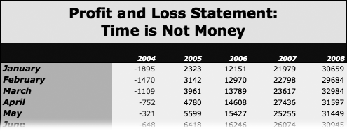
Figure 13-11. Because Excel treats merged cells as one big cell, you can align the contents of that cell any way you’d like; you don’t have to stick to the grid system imposed by a sheet’s cells. One typical use for this is centering a title over a series of columns. Without using merged cells, centering doesn’t do the job at all. When you merge those cells together and apply center alignment, the title is happily centered over the table.
Although you probably won’t want to use Excel as a substitute for Photoshop (and if you do, you have to be seriously creative), you can add graphics and even movies to your sheets and charts. Plus, if you’re artistically inclined, you can use Excel’s drawing tools to create your own art.
When using Excel for your own internal purposes—analyzing family expenditures, listing DVDs, and so on—the value of all this graphics power may not be immediately apparent. But in the business world, you may appreciate the ability to add clip art, fancy legends, or cell coloring (for handouts at meetings, for example). You can even add short videos explaining how to use certain features of your product—or even of the spreadsheet itself.
Although you can add text to cells, and merge cells to create larger text cells, you may often find it helpful to add larger blocks of text to a spreadsheet for explanatory paragraphs, descriptions of your services, or disclaimers reminding your clients that past performance is no guarantee of future results. Enter the Text Box, a mini text document or sidebar that you can place anywhere in a spreadsheet.
Excel gives you two ways of embellishing your spreadsheets with graphic elements of all kinds, the Insert → Picture submenu, and the Object Palette. All these tools work precisely as explained in depth in the Word section of this book.
When you add one of these graphic objects to Excel, it floats on top of the grid rather than inside a cell. You can resize and reposition these objects—and you’ll usually want to position them over empty cells. However, Excel lets you cover up any parts of your spreadsheet data with these graphic objects without so much as a warning murmur. Consider yourself forewarned.
Objects in Excel spreadsheets feature a couple of extra options (or properties) you won’t see in Word or PowerPoint. Since you’re often adding rows and columns to spreadsheets as you work, graphic objects in Excel move along with whatever cells they happen to be sitting on top of. (If they didn’t, you’d risk inadvertently covering your data-filled cells with a picture as you add new columns, for example.)
But if you don’t like this behavior, you can change it—you can fasten the objects to a place on the page instead of in the cell grid. Here’s how: Select the object and choose Format → Picture (or Object, Shape, or Text) and click the Properties tab, and then choose one of the three Object positioning buttons:
Move and size with cells. This option keeps the object tied to the cells beneath it no matter how many columns or rows you add in front of it in the spreadsheet. Additionally, if you resize the columns or rows under this object, it automatically resizes along with them, so it always covers the same number of cells.
Move but don’t size with cells. This option keeps the object tied to the cells beneath (it’s actually locked to the cell that its upper-left corner touches) it but the object remains the same size no matter how you resize the columns or rows beneath it.
Don’t move or size with cells. This option connects the object to a spot on the page, completely ignoring the cell grid. If you add or remove rows or columns the object stays in the same place on the page.
To insert a picture, use the Insert → Picture submenu, which presents five options. Here’s a summary:
Clip Art. This command brings up the Microsoft Clip Gallery, a database containing hundreds of images in 31 categories. You can also search for specific images using the built-in search feature (see Deleting Clips).
From File. Using this option, you can import into your sheet any graphic file format that QuickTime understands, including EPS, GIF, JPEG, PICT, TIFF, or Photoshop.
Shape. Choose this command to summon the Object Palette’s Shapes pane, from which you can insert many different automatically generated shapes—arrows, boxes, stars and banners, and so on (see AutoShapes and WordArt).
Organization Chart. When you choose this menu item, Excel launches the Organization Chart application, which lets you create a corporate-style organization chart with ease. (This kind of chart, which resembles a top-down flowchart, is generally used to indicate the hierarchy of employees in an organization. But it’s also an effective way to draft the structure of a Web site.)
WordArt. The WordArt menu command opens the WordArt Gallery. You can add text and apply some wild effects, including 3-D effects, gradients, shadows, or any combination.
The Insert menu works splendidly, but it’s a little slow and stodgy. In Excel 2008 you can add shapes, clipart, symbols, and photos with a quick click on the Object Palette. To access them, click the Object Palette button in the Toolbox. The palette is divided into four sections—an objects section and a graphics section. The object section includes:
Shapes. This palette lets you add any of Office’s AutoShapes (see AutoShapes and WordArt).
Clip Art. Click this tab to quickly access Office’s collection of clip art and stock photos—although it’s not as complete or searchable as the Clip Gallery accessed by choosing Insert → Picture → Clip Art (see The Clip Gallery).
Symbols. Adds the © (copyright) symbol and scores of other possibilities, saving you a trip to the Insert → Symbol dialog box (see the box on Line Numbers).
Photos. This tab provides a shortcut to your iPhoto collection or any other folder full of photos. (See The Object Palette).
Choose Insert → Movie to open the Insert Movie dialog box with which you can locate any QuickTime movie on your Mac to make part of your worksheet. Select it, and then click Choose. The movie appears with its upper-left corner in the selected cell. You can then resize and reposition it, and then double-click the cinematic masterpiece to play it (see Converting object style). You can insert a sound file in exactly the same way—it lands on your spreadsheet as a loudspeaker icon.
Choose Insert → Text Box; Excel transforms your cursor into a letter A with a crosshair icon. Drag it diagonally anywhere on your spreadsheet to create a text box. When you release the mouse button, the insertion point begins blinking inside, awaiting your text entry. Move your cursor toward any of the text box’s edges until it takes on a four-arrow shape—then you can drag and reposition the box. Surprisingly, unlike text boxes in Word, Excel text boxes feature the green rotating handle sprouting from their top. Drag it to rotate the box.
Excel text boxes are ready for text editing with one click. If you want to change the look of the text box itself—its fill color, line, shadow, and so on—you have the entire Formatting Palette at your disposal (see The Formatting Palette).
If you don’t want to take the time to format the appearance of a text box one element at a time, try the Formatting Palette’s Quick Styles and Effects pane. Click one of the six effects tabs, and then click one of the style thumbnails to apply it to your text box. You can combine the effects to quickly create various 2-D and 3-D effects using shadows, reflections, glows, and so on (see Shadow Tab).