
3
Wind resources for offshore wind farms
Characteristics and assessment
Abstract
The wind resource assessment process characterizes the atmospheric environment through the application of industry-accepted measurement and modeling techniques. The goal is to address wind farm design and performance issues that arise during the development, construction, and operations phases. These issues relate to site selection, energy production estimation, turbine suitability and array layout, the balance-of-plant design, site accessibility, and other project elements. This chapter describes the nature of offshore wind regimes and related phenomena such as sea breezes, internal boundary layers, and tropical cyclones. It also provides a detailed survey of essential resource data parameters and observational approaches using measurement techniques ranging from satellite imagery and conventional fixed-tower platforms to floating lidar. Numerical models are described that assimilate observed data and simulate atmospheric and oceanographic conditions across a spectrum of time and space scales. The performance of turbine wake models is evaluated. Finally, future trends in resource assessment are summarized.
Keywords
Extratropical cyclone; Large-eddy simulation; Lidar; Marine atmospheric boundary layer; Mesoscale models; Metocean; Microscale models; Numerical weather prediction model; Reanalysis; Sea breeze circulation; Thermal stability; Tropical cyclone; Turbine wake models; Turbulence intensity; Wind shear3.1. Key issues in assessing wind resources
The wind is the fuel that wind turbines tap into to generate both electricity and revenue. The wind is also one of the environmental forces that offshore wind farms must endure to perform reliably over their planned lifetime. Wind resource assessment is the process of characterizing the atmospheric environment through measurement and modeling to address the many questions raised during the development, construction, and operational phases of a wind farm. These questions relate to site selection, energy production potential, turbine suitability and layout, the balance-of-plant design, site accessibility, and other project elements.
Air temperature, precipitation, humidity, pressure, and other atmospheric variables are integral to wind resource assessment. They influence both the amount of power available in the wind as well as the efficiency by which wind turbines capture and covert this power. Ocean waves, currents, surface temperature and other water-related parameters are influencing factors too. Not only do they impose major loads on foundations and challenges to vessels, they also directly influence the nature of the overlying atmosphere. Ultimately, the study of the physical and operating design environment of wind farms must be approached in an integrated fashion; meteorological and oceanographic (metocean) factors are interactive. For example, it is the concurrence of extreme winds and extreme waves from severe storms that can define the design envelope to which wind farms must be designed. Fig. 3.1 illustrates many of the metocean factors with which offshore wind turbines must contend.
The greatest challenge to offshore resource characterization is the marine environment itself. Physical measurements are logistically difficult and expensive, which explains why they are relatively sparse. To compensate, strong emphasis is placed on weather satellites and numerical weather prediction models to characterize the ocean environment for many marine activities. While they are effective for special purposes, such as navigation and commercial fishing, their value is more qualitative than quantitative for wind energy applications. This is because the layer of the atmosphere relevant to large-scale wind turbines—extending at least 150 m above the water surface—is not addressed by most measurements, which focus on the ocean surface and a few meters above and below it. Further, because wind turbines are attached to sea bottom-fixed or floating foundations, measurements of the water column, which are largely absent from observational networks, are essential too.

3.2. The nature of the offshore wind environment
Among the most obvious distinctions of the open ocean environment relative to land is the low surface roughness and the lack of terrain. Generally speaking, this contributes to stronger winds with greater horizontal uniformity, smaller changes of wind speed with height (ie, wind shear), and lower levels of turbulence. Fig. 3.2 depicts mean wind conditions over the world's ocean derived from satellite imagery. A surface roughness length of approximately 0.001 m is representative of a sea surface with small waves; by comparison, most vegetated land surfaces have a roughness length of 0.03–1.0 m, depending on the vegetation type and height. Surface roughness length represents the bulk effects of surface roughness elements and has a value of approximately one-tenth the height of those elements (Sutton, 1953; Stull, 1988).
IEC-specified operational conditions for offshore wind turbines assume a power law wind shear exponent of 0.14, with a lower value of 0.11 specified for extreme conditions (IEC, 2009). In actuality, wind shear varies with atmospheric conditions, and average values between 0.06 and 0.16 have been observed in the North Sea and western Atlantic (Berge et al., 2009; Brower, 2012). Typical wind shear values over land average significantly higher: 0.14–0.30. Turbulence intensity (TI), which is defined as the standard deviation of wind speed samples relative to the recorded mean, is commonly observed in the offshore environment to average in the range of 0.05–0.10. High waves produced by strong winds will increase the surface roughness, which in turns increases the TI. TI values are essentially twice as high over land.

Figure 3.2 Wind power density over the global oceans in winter and summer. Source: nasa.gov.
Close to coastlines and islands, land influences on offshore winds grow in importance and come in many forms. When the wind has an offshore component, a transition zone within the marine atmospheric boundary layer (MABL) is created that can extend seaward for several or tens of kilometers. This transition zone, also known as an internal boundary layer, begins at the land–water interface and propagates the land's shear and turbulence traits downwind until they are eventually mixed away (see Fig. 3.3). Winds blowing over long distances parallel to a coastline, particularly one comprised of high terrain, can be channeled to form a coastal barrier jet, which is a zone of higher-speed winds than would otherwise develop if the coast were not present. Flows between islands tend to concentrate the wind and generate higher wind speeds, while lighter winds are experienced both upwind and downwind of the islands due to their barrier effect.

Figure 3.3 Illustration of an internal boundary layer formed as wind blows from land to ocean. Source: Delft University of Technology OpenCourseWare.
The contrast in temperature between the water surface and the overlying atmosphere is an important feature of the ocean environment. This contrast impacts the stability, or the vertical mixing tendency, of the MABL. When warm air moves over cooled water, as often occurs in spring and summer in the middle latitudes of the northern hemisphere, the lower layers of the MABL become thermally stable, or less buoyant. The resulting suppression of mixing leads to stratification and the decoupling of upper air winds from near-surface winds. Sea fog and the suppression of cloud formation are signatures of this condition. This situation can also lead to the formation of low-level jets, which are zones of relatively high wind speeds in the upper layers of the MABL. The depth of a stable layer depends on the duration of the contributing weather conditions, the wind fetch, and other factors, and can be on the order of the height of wind turbines. Consequently, turbine rotors can experience high wind shears during stable conditions, which can last for days or weeks at a time. If the measurement of winds does not probe high enough to represent the entire rotor plane (up to 150–200 m above the surface), these high-shear conditions can go undetected.
The same conditions can cause sea breeze circulations, especially when regional pressure gradients are weak (see Fig. 3.4). This usually occurs under the influence of a high-pressure system and relatively clear skies. During the day, strong solar heating of the land along the coast causes the overlying air to rise. Air over the adjacent water flows inland to replace the rising air, and within a few hours a circulation develops that penetrates deeper inland while drawing in air from distances farther offshore. This phenomenon can enhance offshore wind speeds up to 40 km from shore for several hours, typically from mid-afternoon to early evening; calm zones further offshore can develop as well (Steele et al., 2014). As sunset approaches, the land begins to cool and the sea breeze weakens. Overnight, a reverse but weaker circulation can develop, which is known as a land breeze. The semipermanent Bermuda High is a well-known summer feature that enables frequent sea breeze events in the eastern United States. The coincidence of strong offshore winds when daytime air conditioning loads are highest can be an attractive benefit of offshore wind development in this region (Bailey and Wilson, 2014; Dvorak et al., 2013).

The opposite contrast of air and water temperatures—cold air flowing over warm water—is common in the fall and winter (in the northern hemisphere). This situation creates unstable conditions in the lower MABL, with vertical mixing (thermal convection) that is often earmarked by enhanced cloud formation. Vertical mixing also promotes homogeneity within the MABL, as evidenced by relatively low wind shear. Small air–water temperature differences promote near-neutral stability, which generally occurs most frequently compared to stable and unstable conditions.
Because of water's high heat capacity, the MABL's qualities are slow to change with time compared to the boundary layer over land. The land surface quickly heats and cools during the day and night, causing the stability and wind shear to vary diurnally.
Strong storms deliver the extreme wind and wave conditions experienced in the offshore environment. The two main types of storm systems are tropical cyclones and extratropical cyclones. Tropical cyclones are non-frontal warm-core storms that derive their energy from the release of latent heat of condensation. They originate over warm waters and can assume extratropical characteristics as they move poleward (see Fig. 3.5). Strong tropical cyclones are classified as hurricanes, typhoons, or cyclones—depending on their location—once they attain sustained winds of 33 m/s or greater. Hurricanes occur in the Atlantic and northeast Pacific, typhoons in the northwest Pacific, and cyclones in the South Pacific and Indian Ocean. Tropical cyclones occur with greatest frequency in the summer and early fall seasons when ocean temperatures are warmest.
Extratropical cyclones, which include nor'easter events that occur along the east coast of the United States, have cold-air cores and frontal features, and derive most of their energy from the temperature contrast between different air masses. They can originate over land as well as water. Peak winds can reach hurricane strength. Extratropical cyclones are often larger in radial size than tropical cyclones, with strong winds extending further from the storm center. They occur with greater frequency than tropical cyclones and prevail from mid-fall through mid-spring. Because extratropical cyclones involve colder air temperatures, they can also involve more precipitation types, which in frozen form can accumulate on structures and blades.
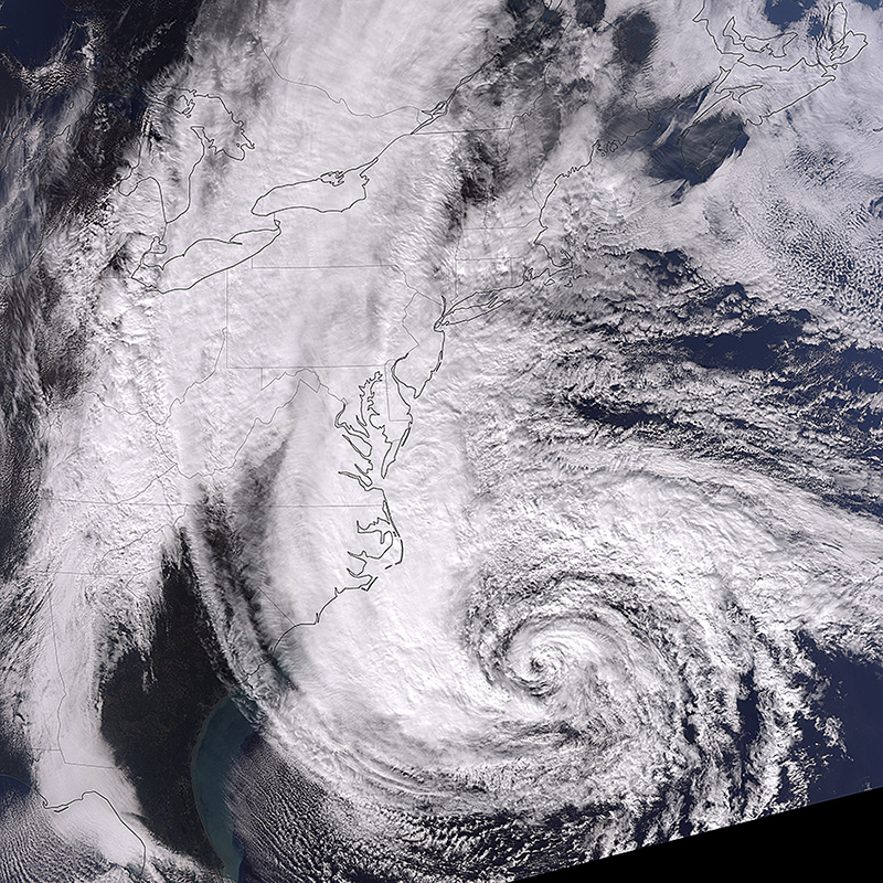
Figure 3.5 Satellite image of northbound hurricane Sandy, October 28, 2012, which became an extratropical storm. Source: earthobservatory.nasa.gov.
3.3. Essential data parameters
Sound planning and design of offshore wind plants depend on a thorough understanding of the local metocean environment. This environment is comprised of a spectrum of atmospheric and oceanographic conditions that vary in time and space. The nature of these conditions, including the extremes that may be encountered over a plant's lifetime, must be addressed in advance to ensure the plant's reliable long-term delivery of energy and storm survivability. The data parameters used to define metocean conditions can be grouped into three categories: wind and other meteorological variables; water- and sea bed-related variables; and joint characteristics. Some parameters are measured directly while others are derived from one or more observations.
The parameters identified in this section reflect the recommendations obtained from a cross-section of leading international standards and guidelines, industry best practice documents, turbine manufacturer suitability forms, and other industry experience (IEC, 2005a,b, 2009; ABS, 2013a,b; ISO, 1975; API, 2007; DNV, 2013). However, differences exist among these sources in terms of parameter measurement and modeling approaches, analytical methods, and time scales.
3.3.1. Wind and other meteorological variables
Within the atmosphere, the measurement of horizontal wind speed and direction is of paramount importance, especially at the intended turbine hub height and ideally at multiple heights, including across the height span of the turbine rotor. The differences in wind speed and direction with height lead to the derivation of wind shear and wind veer, respectively. Standard wind measurement protocols employ a sampling rate of 1–2 s and a recording/averaging interval of 10 min. The standard deviation of sampled speeds within each averaging interval divided by the mean speed for the same interval yields the turbulence intensity (TI), which is another derived parameter. Extreme gusts are derived from the sampled data; statistical methods such as the Gumbel Generalized Extreme Value are used to estimate extreme values for given return periods (typically 50 and 100 years).
Other important direct measurements of the atmosphere include air temperature, atmospheric pressure, and relative humidity. All three are used to determine air density, which directly impacts turbine performance; as such, they should be measured at turbine hub height. However, if this is not feasible, height adjustments can be made using simple assumptions. Relative humidity and temperature also influence the corrosion potential of materials and coatings. Air temperature is also a factor in determining the probability of a turbine exceeding its safe operating and survival envelope (Stout, 2013). The vertical profile of temperature can be used to estimate the thermal stability of the atmosphere, as can the temperature differential between the sea surface and the overlying air.
For cases where wind and other meteorological variables are not observed at hub height, extrapolation techniques are available to adjust values from other heights. For example, measured wind speeds can be adjusted to hub height using the logarithmic wind profile assumption or the power law using an appropriate shear exponent. Both extrapolation techniques are sensitive to the atmospheric stability and work most reliably under near-neutral stability conditions. To minimize the uncertainties associated with extrapolation, measurements should be taken as close to the desired height as possible.
Additional weather variables that can impact wind farms and their operation include precipitation, solar radiation, lightning, and visibility. Precipitation comes in many forms—rain, freezing rain, hail, snow, etc.—and can impact turbine performance, such as from ice buildup on blades. Solar radiation data can be used to approximate blade deterioration rates and for sizing ancillary power supplies; it can also be an input for some atmospheric stability classification methods. Lightning frequency and characteristics data are useful in estimating damage and downtime risks. Visibility data are relevant to wind farm navigation marking requirements, for assessing visual impacts from shore, and to support vessel operations for construction and operations.
Table 3.1 lists recommended meteorological data parameters to be measured and derived. Most nonwind meteorological parameters are sampled and recorded at the same frequency as wind data. Cloud-to-ground lightning statistics can be obtained from government- or privately run detection networks. Hurricane/typhoon/cyclone statistics are available from government meteorological offices.
3.3.2. Water- and sea bed-related variables
Waves, currents, and water levels comprise the primary hydrographic parameters. Short-term wave characteristics are given by a wave spectrum, which is used to determine the wave energy contained at varying wave frequencies or directions. These parameters are derived from observations of significant wave height, wave period, and wave direction. Wave steepness and breaking waves are special cases particularly relevant to wave slamming impacts on foundations (Zang et al., 2015; Peng, 2014). A long-term wave climatology is typically derived by fitting a distribution function to data observed at a site, eg, Rayleigh, Weibull, or Gumbel. Extreme value statistics may be calculated using observed parameter measurements together with empirical formulas, or by fitting observations to distribution models and projecting return times based on the observed frequency of events over a given reference period.
Currents within the water column, which can vary with depth, are also referred to as current profiles. A current profile consists of wind-generated near-surface currents; subsurface currents induced by tidal fluctuations, large-scale circulations, or density gradients; and near-shore currents. The water level and its range consist of an astronomical tidal fluctuation and any storm surge. The juxtaposition of the two results in the maximum range of water levels expected at a site.
Other relevant water-related variables include water temperature, density, salinity, conductivity, and ice. The parameters affecting the density of sea water, such as salinity and temperature, also affect the structural loading due to the water flow. In addition, the presence of sea ice and its physical properties can greatly affect structural loading in cold climates.
Table 3.1
Recommended meteorological data parameters

Table 3.2
Recommended oceanographic data parameters

Corrosion potential may be estimated from observation of water chemistry or pollution, and salinity. Water conductivity measurements are frequently used to estimate water salinity, given known or assumed proportions of dissolved salts. Water temperature also affects corrosion rates, in addition to influencing structural loading characteristics through marine growth.
Estimates of storm surge and sea ice properties are ocean surface observations. For all other parameters listed here, observations throughout the depth of the water column are essential for accurately gauging conditions at development sites.
Table 3.2 summarizes the recommended set of oceanographic data parameters relevant to offshore wind farms.
3.3.3. Joint characteristics
The combination of concurrent metocean factors drives the design loads analysis process as well as the wind farm's turbine layout and energy production. Several combinations of wind–meteorological, wind–water, and water–water parameter analyses are required. For example, one design load condition may evaluate the coincident severe wave height and wind speed. Another may evaluate fatigue loading under conditions when wind and wave directions vary from each other. A wind farm's layout is strongly influenced by the joint speed-direction frequency distribution, which is used to optimally arrange and space turbines in order to minimize production losses due to wakes. Wind turbine output is a function of three coincident factors: wind speed, air density, and turbulence intensity.
Table 3.3 lists relevant joint metocean parameters. The desired parameters, their applications, and the available measurement and modeling technologies will likely expand over time, so it is imperative to remain abreast of offshore wind industry developments and new data needs.
It is worth noting that many of the parameters presented in Tables 3.1–3.3 are common to multiple references, recommended practices, and applications; however, the means of measuring, calculating, and/or analyzing them can vary significantly. Design standards and guidelines provide procedures for certain parameters where consensus or industry best-practices are available. Among these references, however, differences exist in procedures and requirements, and many do not address all parameters equally. Some meteorological parameters, for example, may be called out as relevant for design consideration, with no guidance on how to collect, analyze or interpret them. In other cases, characteristics of certain metocean parameters—relevant measurement frequency, return period, extrapolation method, etc.—will be affected by project location and application.
3.4. Observational approaches
The measurement of offshore wind conditions poses particular challenges due to the hostile marine environment and the need for suitable platforms from which to take reliable observations. Historically, moored weather buoys have comprised the primary source of in situ wind measurements in offshore locales (see Fig. 3.6). They are commonly operated and maintained by government organizations to report on wind, wave and other metocean conditions at strategic locations for purposes of ocean navigation, search and rescue operations, and scientific research. However, their relatively sparse distribution and near-surface wind measurement height (typically 3–5 m above the water surface) limits their value for offshore resource assessment purposes since turbine hub heights are in the vicinity of 100 m.
Weather data collected by moving ships are another source of marine data. The data are transmitted to various national meteorological services as part of the World Meteorological Organization's Voluntary Observing Ships (VOS) program (www.vos.noaa.gov). Approximately 4000 ships participate in the program today, which is down by almost half from the peak of participation in the mid-1980s. Data are heavily concentrated along the major shipping routes in the North Atlantic and North Pacific Oceans. The quality of wind observations from ships is highly suspect because they can be recorded from visual estimates of sea state using the Beaufort scale, from observed wind effects on shipboard objects, or from anemometry which can be strongly influenced by the ship's superstructure.

Figure 3.6 National data buoy center discus buoy located off the coast of Georgia, USA. Adapted from: PMEL Carbon Group http://www.pmel.noaa.gov/co2/.
Oil rigs are another source of offshore wind data, but they are concentrated in certain regions of the world, such as the North Sea and Gulf of Mexico. Only a fraction of rigs maintain continuous wind measurements, and studies have shown that measurement quality is compromised due to the distortion effects of the platforms on the wind field (Berge et al., 2009). Consequently, rig data should be applied with caution.
3.4.1. Satellite
Since the late 1980s, specialized weather satellites have provided information about the ocean's surface winds. These mostly polar-orbiting satellites use microwave sensors to derive surface wind motions by detecting the amount of microwave radiation emitted or reflected by small wavelets. Because the wind is primarily responsible for the creation of these wavelets, methods have been developed to relate microwave observations to surface wind conditions. Weather buoys have been used as the main standard of comparison from which to derive statistical relationships between observed wind conditions and microwave measurements.
There are three main types of sensors used on satellites that detect ocean winds. Passive microwave radiometers measure different microwave frequencies which are passively emitted from the ocean's surface. The spatial resolution is on the order of 25 km, which limits the ability to resolve winds within this distance of a coast or island due to the corrupting influence of land. The first satellite of this type—SSM/I—was launched in 1987 by NASA, and several others have been launched since. Other satellites of this type include TMI, AMSR-E, and WindSAT.
Scatterometers are another sensor type which emit microwave pulses at the earth's surface and receive the return signal using a common antenna. Their resolution is also approximately 25 km, which similarly limits their application in the vicinity of coastlines and islands. Satellites using scatterometers include Quick SCAT/Sea Winds and ASCAT/METOP-1.
The third sensor type, which also actively emits and receives pulses, is synthetic aperture radar (SAR). In addition to surface wind definition, this technology is also used for wave measurements, oil spill detection, and other applications. SAR has the advantage of much finer resolution (generally 25 m) than the other sensor types and can therefore observe offshore winds close to shore. A disadvantage is that SAR has a much narrower field of view and provides coverage of the same given area less frequently. Satellites using SAR include: RADARSAT-1, ERS-2/SAR, ALOS, and RADARSAT-2.
In all cases, the accuracy of satellite-derived wind speed estimates at 10 m above the ocean surface is on the order of 1–2 m/s. Extrapolation to heights approaching 100 m introduces significant uncertainty when estimating hub height wind speeds. It should also be pointed out that the frequency of satellite imagery for any one particular area is usually limited to twice a day or less. This frequency does not provide detail about the diurnal nature of the wind. In general practice for offshore wind energy purposes, satellite information is best used as a first-order siting tool and an indicator of regional wind speeds.
3.4.2. Measurements
Apparent from the foregoing discussion about existing marine wind measurements should be that they are unsuitable alone for characterizing the wind conditions for proposed offshore wind projects. This database of knowledge should therefore be regarded as guidance to facilitate project siting, first-order energy production estimation, and regional wind flow modeling. Investments in new measurements that are tailored to the needs and locations of offshore wind projects are a prerequisite to new project development.
Purpose-built meteorological towers are the primary method for measuring site-specific wind conditions at a proposed offshore project site. The most common design is a self-supporting lattice structure, as shown in Fig. 3.7(a); Fig. 3.7(b) depicts an alternative tapered tubular design. The objective of these structures is to provide a safe and stable platform from which wind, ocean, and meteorological data can be taken for one or more years. Below the tower portion is a foundation section that is attached securely to the seabed. In addition to a large suite of sensors and mounting booms, the towers must also accommodate other features: a power supply (including battery storage), data logging and communications equipment, aviation obstruction lighting, aids to navigation, docking capabilities, biological monitoring systems, and personnel safety features. The entire tower system must be designed to withstand hurricane force winds, extreme waves and currents, and ice loading. Corrosion of structural steel must be addressed, as must the potential for scour in the design of the foundation.

Figure 3.7 (a) FINO3 platform with 100-m lattice-type tower. (Source: fino-offshore.de.); (b) Cape Wind platform with 60-m tapered tubular-type tower. (Source: AWS Truepower LLC.)
International standards do not yet exist to specify how offshore wind measurements must be taken, but industry best-practices encourage high levels of redundancy and sensor robustness to ensure reliable data capture. For example, three sets of anemometry are recommended for each measurement level, as opposed to two sets for land-based measurements, to achieve the desired target of 90% or greater data recovery. This is because offshore environments are harsher and more difficult to access when maintenance is required. Offshore towers are also more massive and, consequently, more likely to experience flow distortion issues. Sensors extending off of multiple faces of a tower can facilitate the detection and subsequent correction of flow distortions. IEC specifications (IEC 61400-12-1) recommend that wind sensors be placed on booms extending at least three to six tower widths away from the sides of towers, depending on tower solidity, to minimize distortion effects.
While wind measurement programs for land-based wind projects employ multiple towers, offshore projects will most likely invest in at most one. For the most part, this is because of the high cost of an offshore tower ($10 million ± 50%, depending on locale and other factors), which is roughly two orders of magnitude greater than a typical land-based tower. Another consideration is that the need for multiple towers is much less justified offshore because of terrain and surface roughness uniformity within proposed project areas. In practice, a singular tower is usually positioned just outside, and upwind of, the perimeter of the proposed turbine array. This placement allows the tower to continue supplying useful observations even after the array is installed and commissioned. Numerical modeling is used to extrapolate the tower's observed conditions throughout the project area.
The high cost of offshore towers and the practical limits of their installation in waters deeper than approximately 40 m have opened the door to alternative measurement approaches. The leading candidate is profiling lidar, which can be mounted on fixed or floating platforms; sodar has been used on occasion but is suitable only on fixed platforms. On fixed platforms (such as short towers or jack-up barges), measurements taken by either remote sensing technology have shown a high degree of comparability and correlation with concurrent wind observations taken from adjacent tall towers (Cox, 2014; Hung et al., 2014; Barthelmie et al., 2003). These technologies can complement tower-based measurements by sampling winds above the top of the tower, such as across the upper portion of the turbine rotor span.
Unless an existing fixed platform is available, it may be cost-prohibitive to invest in a new, purposely built one to support lidar or sodar. Buoy-mounted floating lidars (see Fig. 3.8) are now commercially available that have demonstrated the ability to measure winds aloft with essentially the same accuracy as tall-tower measurements. However, more extensive validations on long-term measurement reliability are needed before the offshore wind industry fully accepts floating lidar as a replacement for tall towers. A drawback to reliance on lidar data alone is that, unless more than one colocated lidar is used, there is no backup measurement system should there be an operational problem. Furthermore, lidar is unable to measure temperature profiles, which can readily be observed from a tall tower.
A measurement period of at least one full year, and preferably two or more, is required to understand the magnitude and variability of winds and other conditions across all seasons. Compared to the 20+ year life of a wind project, this duration is relatively short and will not adequately represent long-term conditions. The measure-correlate-predict (MCP) method is commonly used to derive a long-term climatology of wind conditions from the onsite observations. The MCP process works by correlating the site's wind observations with concurrent data from a high-quality long-term reference located within the same region, such as a coastal weather station or model-generated reanalysis grid data. The established relationship (such as a regression equation) between the two is then applied to the reference's historical record to predict the long-term average wind characteristics for the project site. This approach assumes, of course, that the past is a reliable indicator of the future. This has been found to be generally true within an uncertainty margin of approximately 2% for well-correlated sites (r2 > 80%) where the duration of the reference station's wind records is at least 10 years (Brower, 2012).

The lack of available wind speed measurements at or near the hub height of modern offshore wind turbines contributes significant uncertainty to wind speed estimation. The majority of publicly available offshore wind data are collected by buoys at anemometer heights of 5 m or less. Satellite-derived estimates of ocean winds are available at a 10 m height. Fig. 3.9 shows a broad range in hub height speed estimates that would result from using a range of power law shear exponents to extrapolate a known wind speed value from 5 m above the surface up to 120 m. The 5-m wind speed value of 6.7 m/s was the measured annual average observed by a north Atlantic buoy in 2013, while estimated 80-m wind speeds varied from 7.5 to 11 m/s. The average shear exponents represent a range of values that are representative of an offshore environment:
• 0.05: Extreme storm conditions, such as Nor'easters
• 0.08: Low end of mean annual offshore wind conditions
• 0.11: IEC-specified shear for extreme conditions for offshore wind turbines (IEC, 2009)
• 0.14: IEC-specified operational conditions for offshore wind turbines (IEC, 2009)
• 0.17: Mean annual near-shore wind conditions (high offshore value)
Because the shear exponent that should be used cannot be precisely determined without directly measuring the shear, and the shear may also change with height, buoys or satellite-based estimates alone are insufficient for deriving reliable information about hub height wind conditions.

3.5. Modeling approaches
Numerical modeling is commonly used to assimilate disparate sources of observed data to create an integrated approximation of atmospheric and oceanographic conditions within a defined time and space domain. It is commonly applied to produce weather maps, forecasts, and other products to serve the needs of the general public as well as specialized industries. The skill of numerical models for analysis and forecasting applications has advanced dramatically in recent decades, due largely to huge gains in affordable computing power and to the availability of new data inputs from sources like weather satellites. This section reviews how numerical modeling is used within the offshore wind energy sector to simulate metocean conditions, in particular winds, waves, and currents. The discussion will emphasize the modeling of winds, which not only drive the operation of wind turbines but also the generation of most waves and currents.
Meteorological phenomena occur over a wide range of time and space scales. Fig. 3.10 gives an example of atmospheric processes ranging from seconds to weeks, and from meters to thousands of kilometers. The four space scales—microscale, mesoscale, synoptic, and global—refer to the horizontal dimension of atmospheric motions, which range from short-lived microscale phenomena, such as turbulent eddies and wind gusts, to much longer-lasting global long waves and trade winds. All these scales of atmospheric motion interact with each other as well as with the land, the oceans (and other water bodies), and sea ice.
In atmospheric sciences, numerical models are built around the equations of fluid dynamics, namely the Navier–Stokes equations, with varying degrees of complexity (or nonlinearity). The equations may include conservation of mass, momentum, energy, and moisture, as well as an equation of state for air based on the ideal gas law. Numerical weather prediction (NWP) models and large-eddy simulations (LES) solve all of these equations. Due to computational runtime, cost, or other constraints, some (simpler) models solve only a subset of the equations. Although the atmosphere is always evolving and various weather variables are changing in intensity, not all numerical models are able to step forward in time. Prognostic models are ones that simulate the evolution of atmospheric conditions over time, while diagnostic models simulate steady-state conditions.

Models of different types operate at different time and space scales, depending on the application. For example, climate models predict long-term changes in atmospheric properties (such as mean temperature, precipitation, and winds) over large portions of the globe (ie, at the synoptic and global scales). NWP models simulate short-term changes within smaller regions, such as portions of countries (ie, the mesoscale and synoptic scale); this scale is consistent with the size of modern wind farms. Microscale models are applied to processes in even smaller areas, such as within individual wind farms at the scale of individual turbines. Using a finite data set, essentially all models represent the environment with a three-dimensional grid. Most atmospheric models incorporate multiple vertical layers, some extending up to several kilometers in altitude. Grid resolution, particularly in the horizontal dimension, is generally consistent with the model space scale, with much coarser-resolution grid spacing employed by climate models compared to mesoscale NWP models or microscale models.
The selection of grid spacing and domain size in a modeling exercise is critical when attempting to represent the flow phenomena of interest. Physical processes such as turbulence or cumulus clouds that are too small to be explicitly resolved by a model within its grid scale need to be approximated using some sort of parameterization scheme. Physical features such as mountains, islands, or irregular coastlines that are smaller than the model's grid resolution will generally be ignored. A standard strategy to capture small features or small-scale processes with a numerical model is to run a finer-resolution grid nested inside a coarser-resolution grid. Typically, the latter covers a much larger region than the finer-resolution grid (similar to a box inside a box). Grid nesting is used to downscale coarse resolution information to a finer-resolution grid while ensuring proper energy transfers in the atmosphere.
3.5.1. Numerical weather prediction models
NWP models have been developed primarily for weather forecasting purposes over different time horizons ranging from hours to days. These models heavily rely on observations of initial surface and atmospheric conditions, which include surface weather stations, buoys, ships, radiosondes (weather balloons), radars, aircraft, and satellites (visible, infrared, and microwave bands). Mesoscale NWP models are well-equipped for simulating wind flows accurately in offshore environments. Several studies have demonstrated their ability to represent many of the complex wind phenomena found in offshore environments: mountain and island blocking, gap flows, coastal barrier jets, internal boundary layer growth, stability transitions, sea breeze circulations, and so on (eg, Colle and Novak, 2010; Freedman et al., 2010; Steele et al., 2013; Gilliam et al., 2004). The root mean square error (RMSE) of wind speed data from NWP models is typically around 2–3 m/s in offshore regions (Jimenez et al., 2007; Berge et al., 2011; Beaucage et al., 2007; Dvorak et al., 2010). In addition to wind speed components at several heights, NWP models can output almost any atmospheric variable.
The typical model resolution for most mesoscale simulations is on the order of a few kilometers, ie, near the interface between the microscale and mesoscale. Since this scale does not provide a very detailed picture of wind conditions within a large wind farm, coupling with a microscale model is often done to obtain the desired detail. It has been demonstrated that a coupled mesoscale NWP and microscale model shows improvement over a mesoscale model alone. Examples of coupled mesoscale and microscale models include AWS Truepower's MesoMap and SiteWind systems (Brower, 1999), Risø National Laboratory's KAMM-WAsP system (Frank et al., 2001), and Environment Canada's AnemoScope system (Yu et al., 2006). Coupled model approaches have been used to create relatively high-resolution wind maps and atlases of the globe. Fig. 3.11 is a representation of the annual average wind speed of the United States, including a 90-km wide zone of offshore winds, at 100 m above the surface at a spatial resolution of 2 km (Elliott et al., 2010; Schwartz et al., 2010). In northern Europe, the NORSEWIND (NORthern Seas Wind Index Database) project, which began in 2008, has develop wind atlases for the Irish Sea, the North Sea, and the Baltic Sea using offshore wind measurements, satellite data, and numerical model data (Hasager et al., 2010).
Mesoscale models take into account subgrid scale effects and physics parameterizations for solar radiation, land surface–atmosphere interaction, the planetary boundary layer (PBL), turbulence, cloud convection, and cloud microphysics. Since they incorporate the dimensions of both energy and time, NWP models are capable of simulating such phenomena as thermally driven mesoscale circulations (eg, sea breezes, thunderstorms) and atmospheric stability, or buoyancy. In the world of mesoscale modeling—as in the real world—the wind is never in equilibrium with the surface because of the constant exchange of energy. This exchange occurs through solar radiation, radiative cooling, evaporation and precipitation, and the cascade of turbulent kinetic energy down to the smallest scales.

Figure 3.11 Annual average US wind speed at 100 m above the surface, land-based and offshore. Source: nrel.gov/wind/resource_assessment.
In addition to forecasting weather conditions, NWP models are useful in predicting atmospheric conditions for historical periods, ie, looking backwards in time. This practice is sometimes referred to as “hindcasting” and has the capability of assessing regional wind conditions from existing long-term datasets before launching new measurements at an offshore site of interest. A number of mesoscale gridded datasets are now available on a global basis from various sources spanning several decades. Referred to as “reanalysis,” these datasets have been compiled using a fixed data assimilation approach and NWP model with the primary goal of removing potential biases or artificial trends resulting from the gradual changes in modeling approaches, observation types and regional data collection concentrations over the decades (Kistler et al., 2001). For example, from the 1940s to the 1970s, weather observations were primarily derived from fixed surface weather stations, buoys, weather balloons, ships, and aircraft. Beginning in the 1970s, satellite-based observations of cloud-tracked winds and other parameters began, and since then significant increases in the number of satellites and types of onboard sensors have made satellites the dominant environmental data gatherer across the globe. Even among the nonsatellite types of measurement systems, over time there have been large changes in the density and number of surface and upper air observations, improvements in the quality of the data collected, and the introduction of new data-recording and -sensing technologies and the retirement of old ones. Reanalysis datasets, therefore, provide the most consistent records of atmospheric conditions over long periods of time.
The original reanalysis dataset is known as the National Center for Environmental Predictions/National Center for Atmospheric Research (NCEP/NCAR) Reanalysis 1 (Kalnay et al., 1996). It covers the period from 1948 to present at a spatial resolution of 1.87 degree (approximately 205 km). Since then, several national meteorological agencies and national research laboratories including the European Center for Medium-Range Weather Forecasts (ECMWF), NCEP, National Aeronautics and Space Administration (NASA), and the Japanese Meteorological Agency (JMA), have issued their own reanalysis products. These products include the ERA-Interim, Climate Forecast System Reanalysis (CFSR), Modern-Era Retrospective analysis for Research and Applications (MERRA), and Japanese 55-year Reanalysis (JRA-55). They are based on advanced data assimilation schemes and NWP models and have been generating data at a finer spatial resolution of 0.5–0.75 degree (55 or 83 km) than the NCEP/NCAR Reanalysis 1. Reanalysis data are typically available on a 6-h interval, however there are two exceptions: the MERRA and CFSR, which are available hourly for some surface fields and limited pressure levels.
The relatively coarse grid resolution of reanalysis data (50 km or so) can capture offshore wind flows well if the site of interest is located far enough from the coast (or islands) such that the model grid cell does not include any land portion. However, nested, higher-resolution grids can be modeled to simulate near-shore wind circulations. Reanalysis datasets are also valuable for correlating short-term time series measurements collected on offshore platforms with long-term climatological records. Even though the mean bias between reanalysis and meteorological mast data can be substantial, the value of reanalysis data relies mostly in their correlation to onsite measurements, which are not impacted by a bias. Several studies (Brower et al., 2013; Lileo and Petrik, 2011; Decker et al., 2012; Stoelinga et al., 2012) show that the latest-generation reanalysis datasets—for instance, ERA-Interim, CFSR, and MERRA—have superior accuracy in terms of their correlation to mast data.
3.5.2. Microscale models
In order of increasing complexity, microscale wind flow models fall into several broad categories: mass-conserving, linear Jackson–Hunt type, computational fluid dynamics (CFD), and LES. Mass-conserving types are so-called because they solve just one of the physical equations that govern mass conservation. Most mass-conserving models like WindMap (Brower, 1999) and CALMET (Scire et al., 2000) are designed to depart by the smallest possible amount from an initial wind field estimate derived from observations and/or a mesoscale model output. Mass-conserving models are generally not used as standalone models and are often coupled to a mesoscale NWP model. Linear wind flow models like the Wind Atlas Analysis and Application Program (WAsP) (Troen and Petersen, 1989; Troen, 1990), MS3DJH/MsMicro (Taylor et al., 1983), the Mixed Spectral Finite Difference model (MSFD) (Beljaars et al., 1987), and Raptor (Ayotte and Taylor, 1995) are based on the theory of Jackson and Hunt (1975). They go beyond mass conservation to include momentum conservation by solving a linearized form of the Navier–Stokes equations under several assumptions: steady-state flow, linear advection, and first-order turbulence closure. However, they do not take into account any horizontal temperature gradients or flow acceleration.
A version of CFD models known as Reynolds-averaged Navier–Stokes (RANS) models has emerged as an alternative to Jackson–Hunt models for wind energy applications as personal computers have grown more powerful. They were designed originally to model turbulent fluid flows for airplane bodies, jet engines, and the like. Several RANS models are being used in the wind energy industry: Fluent, CFX, Star-CCM+, OpenFOAM, Meteodyn WT, WindSim, Ventos, etc. The critical difference between RANS and Jackson–Hunt models is that the former solve the nonlinear Navier–Stokes momentum equations, but none of them includes the full conservation of energy equation. The RANS models assume steady-state flows. LES are a promising alternative to RANS models in that they explicitly resolve the energy-containing eddies—those larger than the grid spacing—while simulating the effects of smaller turbulent eddies through a subgrid scale parameterization scheme. LES models are mainly used as a research tool since the necessary computing power is huge. LES can include the full suite of physics parameterization schemes: radiation, microphysics, land surface–atmosphere interaction, turbulence, etc. LES models are based on the raw equations of motion, ie, unsteady, nonlinear Navier–Stokes equations. A fundamental difference between LES and RANS models is that LES solve the conservation of energy equation, which allows LES to fully capture the wind circulations forced by thermal gradients, which is an important driver of offshore wind flows. LES are designed to run at very fine spatial resolutions using a grid spacing in the 1–100-m range. To date, LES have been rarely used to determine the offshore wind resource due to their computational expense and the fact that NWP and microscale models tend to perform relatively well when dealing with the average wind speeds across a large area. However, there is a growing interest for LES to capture the unsteady and nonlinear turbine-induced wakes as well as their two-way interactions with the boundary layer (Jimenez et al., 2007; Calaf et al., 2010; Churchfield et al., 2012).
3.5.3. Modeling of turbine-induced wakes
While the foregoing discussions about models have focused on the representation of atmospheric conditions at different space and time scales, another modeling problem is the understanding of distortions within these conditions when wind turbines are added to the modeling domain. These distortions are commonly referred to as wakes, which are comprised of turbulent eddies shed by the turbines' blades, nacelle, and tower. As turbulence sources and momentum sinks, upwind turbines within an array reduce the energy output and increase the structural fatigue of downwind turbines. Energy production losses in large wind farms due to the compounding effects of wakes caused by multiple turbine rows can exceed 15–20% if not properly arranged. The importance of turbine-induced wakes for offshore wind projects is not limited to wake losses due to individual turbines; the entire wind farm can impact neighboring wind farms. This latter effect is sometimes called wind farm shadowing.
Historically, wake-effect predictions have been based on a handful of engineering computer models, most importantly Park (Katic et al., 1986; Jensen, 1983) and eddy viscosity (EV) (Ainslie, 1988). The Park model implements a simple formula for the size of the wake deficit and its expansion downstream with a single adjustable parameter, the wake decay constant. The EV model solves an axisymmetric form of the Navier–Stokes equations; it therefore qualifies as a simple RANS model. With the development of large-array wind projects, it has been found that the standard Park and EV models tend to underestimate wake losses in offshore wind farms (Brower and Robinson, 2009; Schlez and Neubert, 2009; Barthelmie et al., 2010). This may be in part because the models assume that wind turbines have no effect on the planetary boundary layer (PBL) other than the wakes they directly generate. As a consequence, new codes have been developed to account for two-way PBL–wake interactions such as the Deep-Array Wake Model (DAWM) in Openwind (Brower and Robinson, 2009) and Large Array Wind Farm (LAWF) model in WindFarmer (Schlez and Neubert, 2009). The DAWM is based on the surface-drag-induced internal boundary layer approach which modifies the wind speed profile within the PBL with increasing distance downstream of the front of a turbine array. The EV or Park model is retained for estimating direct wake effects, thus the term hybrid model. The LAWF model (Johnson et al., 2009) is an extension of standard wake models whereby each turbine is treated as a disturbance analogous to a roughness element that influences the free stream flow, resulting in growth of the internal boundary layer. Both approaches are commonly used today and have demonstrated significant improvement over the original models (Beaucage et al., 2012; Brower and Robinson, 2009).
Another relatively new type of engineering model capable of predicting the turbine-induced wakes is the dynamic wake meander (DWM) model, which is a more detailed model of the flow field behind the upstream turbine (Larsen et al., 2012). This method applies a meandering process within an aeroelastic code in order to simulate the incoming flow field at downstream turbines and calculate both energy production and loading. The Fuga model (Ott et al., 2011) is a linearized RANS model that inserts an actuator disk (an idealized model of a wind turbine rotor's effect on the airflow) to simulate the wakes. It bears some similarities to WAsP, including a mixed spectral solver using precalculated look-up tables. Another relatively new commercial RANS model is WindModeller based on Ansys CFX (Montavon et al., 2011). It incorporates a turbulence closure and an actuator disk. LES models have recently been used to study single and multiple turbine-induced wakes (Wu and Porté-Agel, 2011; Calaf et al., 2010; Churchfield et al., 2012; Troldborg et al., 2014; Mirocha et al., 2014). For single turbine-induced wakes, LES models with a wind turbine parameterization using an actuator disk and/or actuator line model can compare favorably to wind tunnel measurements (Wu and Porté-Agel, 2011). LES codes are a promising approach to simulating wakes if a high-performance computing system is available. Both the open-source Simulator for Offshore/Onshore Wind Farm Applications (SOWFA) from the National Renewable Energy Laboratory (NREL) (Churchfield et al., 2012) and the LES implemented in the WRF model (Mirocha et al., 2014), offer opportunities for the academic and industry sectors to collaborate and develop the next generation of turbine-induced wake models.
A benefit to advancing turbine wake models is to enable turbine and wind farm control systems to optimize operations using wake-related intelligence. For example, under some weather conditions it is possible to enhance overall wind farm output by manipulating (yawing) the orientation of upwind turbines so that their wakes are steered to mitigate negative impacts on downstream turbines. This capability is especially feasible with real-time monitoring of boundary-layer conditions (winds, stability, turbulence) at a wind farm.
In summary, there is a growing number of commercial and research wind turbine wake models but validation datasets from operating offshore wind farms remain limited. Further, those datasets collected by private entities are not typically shared. Because turbine wakes can be a significant cause of power production losses, especially in large arrays, ongoing model advances are desired to optimize wind farm performance through improved layouts and turbine control strategies, and through reduced fatigue loads on turbine structures.
3.5.4. Coupled atmosphere–ocean models
While coupling wind and wave modeling is important, coupling to oceanic models may be even more important since the thermal influences of the ocean on the atmosphere (specifically the impacts of currents, winds and precipitation on sea surface temperature) play a critical role in the response of the MABL. The main benefit of coupling atmospheric, wave and ocean models is balancing the fluxes of heat and momentum at the water surface. Without coupling, closed models tend to develop solutions in unrealistically diverging ways. Coupled wave–ocean–atmosphere models incorporate physics-based parameterizations that can significantly improve simulations and forecasts of wind, waves and currents—including hurricane tracks and intensity—in coastal regimes where air–land–sea contrasts drive mesoscale circulations (Lee and Chen, 2012). In cases where new observations are to be sited with an explicit goal of improving model predictability, modeling techniques are now available that can reveal the measurements types and locations that are most influential in producing a forecast of sufficient accuracy over a given area.
More research focus is needed on processes that couple the turbulent atmospheric and oceanic boundary layers across the interface through the exchange of momentum, mass, and heat. Separate atmospheric and wave models are closed systems that rely on simplified boundary conditions, which can lead to inaccurate solutions. Advancements in the coupling of ocean-atmosphere models will result in increasingly realistic representations of the interplay between the different components of the metocean regime.
3.6. Future trends
As the interest in offshore wind energy spreads geographically, the demand for new measurements of metocean conditions will grow. This trend will spur a new generation of offshore data collection activity and drive measurement innovation. It will also improve our understanding of the MABL in more regions, especially where the new data are shared publicly and the research community is actively engaged.
Floating lidar is one of the measurement innovations likely to succeed. Early field validations against fixed meteorological towers have yielded excellent wind speed data comparisons, and several versions of floating lidar are now commercially available. Motion compensation is either integrated into the data analysis routines or is outright unnecessary due to the controlled movement of specially designed weather buoys. Purpose-built buoys like these can support multiple types of metocean sensors together with robust power supplies, battery storage, and communication systems.
The use of meteorological towers is likely to continue for many proposed projects, especially in water depths of under 50 m, because of their inherent benefits. Sensors can be placed at specific heights of interest, and wildlife monitoring equipment can be piggy-backed on the same platforms, making for a multipurpose research facility. Due partly to their cost, offshore wind projects are likely to invest in only one meteorological tower during the development phase. However, complementary floating lidar platforms will likely see greater use because they can be more easily and cost-effectively located and relocated to represent other portions of the planned project area. As a fixed asset, the meteorological tower can remain after the wind farm is built to support ongoing monitoring activities.
Expanded data collection efforts will enable the advancement of ocean and atmospheric models to simulate metocean conditions with greater fidelity across a range of space and time scales. The lack of observations has been the main barrier to comprehending the dynamics of the MABL and accurately predicting the key features with the combination of mesoscale and microscale models. Modeling improvements, including coupled ocean–atmosphere models, will lead to better representations of important dynamic offshore processes. These include complex land–sea–air interactions that influence sea breeze circulations, low-level jets, thermal profiles, and other marine boundary-layer phenomena.
Climate change and its potential impact on the intensity and frequency of storms is a wild card variable. Wind farms are designed to withstand the worst weather conditions expected over their lifetime. The magnitude and return period of extreme conditions is normally derived from historical data. But with warmer ocean temperatures, sea level rises, and increases in atmospheric humidity, the probabilities of stronger storms is rising. Studies have found a correlation between these changes and the destructive power of tropical storms. Climate change must be accounted for in the planning of future offshore wind farms.
Abbreviations
| ABS | American Bureau of Shipping |
| ALOS | Advanced land observing satellite |
| AMSR-E | Advanced microwave scanning radiometer—earth observing system |
| API | American Petroleum Institute |
| ASCAT/METOP-1 | Advanced scatterometer/meteorological operations satellite |
| CFD | Computational fluid dynamics |
| CFSR | Climate forecast system reanalysis |
| DAWM | Deep array wake model |
| DNV | Det Norske Veritas |
| DWM | Dynamic wake meander |
| ECMWF | European Center for Medium Range Weather Forecasts |
| ERA | ECMWF reanalysis |
| ERS-2 | European Remote Sensing Satellite 2 |
| EV | Eddy viscosity |
| IEC | International Electrotechnical Commission |
| ISO | International Organization for Standardization |
| JAM | Japanese Meteorological Agency |
| JRA | Japanese reanalysis |
| KAMM | Karlsruhe Atmospheric Mesoscale Model |
| km | Kilometers |
| LAWF | Large array wind farm |
| LES | Large eddy simulation |
| m | Meters |
| MABL | Marine atmospheric boundary layer |
| MCP | Measure-correlate-predict |
| MERRA | Modern-era retrospective analysis for research and applications |
| Metocean | Meteorological and atmospheric |
| m/s | Meters per second |
| MSFD | Mixed spectral finite difference |
| Table Continued | |

| MS3DJH | Mason and Sykes three-dimensional extension of Jackson–Hunt |
| NASA | National Aeronautics and Space Administration |
| NCAR | National Center for Atmosphere Research |
| NCEP | National Center for Environmental Predictions |
| NORSEWIND | Northern Seas Wind Index Database |
| NREL | National Renewable Energy Laboratory |
| NWP | Numerical weather prediction |
| PBL | Planetary boundary layer |
| QuikSCAT | Quick scatterometer |
| RADARSAT | Radar satellite |
| RANS | Reynolds-averaged Navier–Stokes |
| RMSE | Root mean square error |
| SAR | Synthetic aperture radar |
| SOWFA | Simulator for offshore/onshore wind farm applications |
| SSM/I | Special sensor microwave imager |
| TI | Turbulence intensity |
| TMI | Tropical rainfall measuring mission's microwave imager |
| WAsP | Wind Atlas Analysis and Application Program |
| WRF | Weather research and forecasting |
| VOS | Voluntary observing ships |

..................Content has been hidden....................
You can't read the all page of ebook, please click here login for view all page.