9.3. Filter inductors

Search in book...
Toggle Font Controls
Create new playlist

Name your new playlist

Playlist description (optional)
Sign In

Email address

Password

Forgot Password?

or

Continue with Facebook

Continue with Google
Sign Up

Full Name

Email address

Confirm Email Address

Password

or

Continue with Facebook

Continue with Google

9.3. Filter inductors

9.3.1. Main constraints in the inductor design

The starting point for an inductor design is the stored energy relation (Eq. [9.31]) defined by the inductance L, the inductor peak current (

\hat{I_{L}}

$\hat{I_{L}}$

), the RMS current (I_L), the RMS current density (J_L), the peak flux density (B_L), the winding conductor fill factor (k_wc), the winding window area (A_w) and the core area (A_core) (Mohan et al., 2003).

$L \cdot \hat{I_{L}} \cdot I_{L} = k_{wc} \cdot J_{L} \cdot B_{L} \cdot A_{w} \cdot A_{core}$ $L \cdot \hat{I_{L}} \cdot I_{L} = k_{wc} \cdot J_{L} \cdot B_{L} \cdot A_{w} \cdot A_{core}$

[9.31]

The product (A_w·A_core) appears in Eq. [9.31] and is an indication of the core size and it is called area product. For a given core material, the peak flux density is limited by the saturation flux density (B_sat). A similar situation is given for the winding conductor, which physically limits the maximum current density (J_max) of the inductor winding. Even more, if a conductor type and core type are fixed for the inductor design, the winding conductor fill factor becomes approximately a design constant.

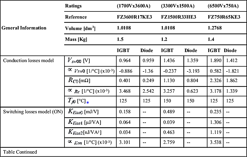
Table 9.2

Semiconductor Parameters; IGBT modules from Infineon manufacturer for three different voltage ratings are considered.

General Information	Ratings	(1700Vx3600A)		(3300Vx1500A)		(6500Vx750A)
	Reference	FZ3600R17KE3		FZ1500R33HE3		FZ750R65KE3
	Volume [dm³]	1.0108		1.0108		1.2768
	Mass [Kg]	1.5		1.2		1.4
		IGBT	Diode	IGBT	Diode	IGBT	Diode
Conduction losses model	$V_{s w 00}$ $V_{s w 00}$ [V]	0.964	0.959	1.436	1.359	1.890	1.412
	$\propto_{V s w 0}$ $\propto_{V s w 0}$ [1/°C] (x10^-3)	-0.886	-1.36	-0.237	-3.193	0.582	-1.821
	$R_{C 0}$ $R_{C 0}$ [mΩ]	0.401	0.249	1.130	0.804	2.326	1.862
	$\propto_{R c}$ $\propto_{R c}$ [1/°C] (x10^-3)	3.468	2.542	3.257	0.623	3.178	1.339
	$T_{j 0}$ $T_{j 0}$ [°C]∗	125	125	150	150	125	125
Switching losses model (ON)	$K_{E o n 0}$ $K_{E o n 0}$ [mJ/V]	0.158	‐‐	0.489	‐‐	0.235	‐‐
	$K_{E o n 1}$ $K_{E o n 1}$ [μJ/VA]	0.064	‐‐	0.039	‐‐	1.306	‐‐
	$K_{E o n 2}$ $K_{E o n 2}$ [nJ/VA²]	0.034	‐‐	0.463	‐‐	1.119	‐‐
	$\propto_{E o n}$ $\propto_{E o n}$ [1/°C] (x10^-3)	3.101	‐‐	2.759	‐‐	3.538	‐‐
Table Continued

General Information	Ratings	(1700Vx3600A)		(3300Vx1500A)		(6500Vx750A)
	Reference	FZ3600R17KE3		FZ1500R33HE3		FZ750R65KE3
	Volume [dm³]	1.0108		1.0108		1.2768
	Mass [Kg]	1.5		1.2		1.4
		IGBT	Diode	IGBT	Diode	IGBT	Diode
Switching losses model (OFF)	$K_{E o f f 0}$ $K_{E o f f 0}$ [mJ/V]	0.037	0.328	0.116	0.314	0.021	0.185
	$K_{E o f f 1}$ $K_{E o f f 1}$ [μJ/VA]	0.404	0.334	0.731	0.728	1.546	1.118
	$K_{E o f f 2}$ $K_{E o f f 2}$ [nJ/VA²]	0.008	-0.027	0.045	-0.135	0.014	-0.326
	$\propto_{E o f f}$ $\propto_{E o f f}$ [1/°C] (x10^-3)	3.276	4.25	2.435	5.333	1.429	5.333
Parallel connection	$Δ V_{s w}$ $Δ V_{s w}$ [V] at 25[°C]	0.45	0.40	0.55	0.75	0.4	0.5
Parallel connection	$δ_{C I}$ $δ_{C I}$ [%] at T_j,max	18.48	28.72	19.36	26.16	12.95	21.81
Static Thermal model	R_thJC [K/kW]	6.3	14	7.35	13	8.7	18.5
	R_thCH [K/kW]	8.7	19.5	10	11	8.8	14
	N_isxm	3		3		3
	T_j,max [°C]	125		150		125
Switching times	t_on,max at T_j,max [μs]	1.05	‐‐	1.15	‐‐	1.2	‐‐
	t_off,max at T_j,max [μs]	2.1	0.88	3.85	1.73	8.1	2.67
	f_sw,max∗∗ [kHz]	4.96 → 4		2.97 → 2		1.67 → 1.5

When a reduction in the total size of the inductor is targeted for some given electrical parameters, like inductance and current, then the designer should deal with this by pushing the peak flux density and current density as close as possible to the physical limits and thermal constraints, as the product J_L·B_L is inversely proportional to the winding area and the core area. Then, the minimum area product for a given set of constraints can be written as:

$A_{w} \cdot A_{core} \propto \frac{L \cdot \hat{I_{L}} \cdot I_{L}}{J_{max} \cdot B_{sat}} \propto E_{L} \propto L \cdot {I_{L}}^{2}$ $A_{w} \cdot A_{core} \propto \frac{L \cdot \hat{I_{L}} \cdot I_{L}}{J_{max} \cdot B_{sat}} \propto E_{L} \propto L \cdot {I_{L}}^{2}$

[9.32]

9.3.2. Size modelling

Geometrically, it can be shown that the area product is also related to the volume of the inductor by (Mohan et al., 2003):

$A_{w} \cdot A_{core} \propto Vo l_{L}^{4 / 3}$ $A_{w} \cdot A_{core} \propto Vo l_{L}^{4 / 3}$

[9.33]

Combining Eqs [9.33] and [9.32], the overall inductor volume (Vol_L) can be expressed as:

$Vo l_{L} \propto {(L \cdot {I_{L}}^{2})}^{3 / 4}$ $Vo l_{L} \propto {(L \cdot {I_{L}}^{2})}^{3 / 4}$

[9.34]

Then, if an inductor design technology is kept (core material, conductor type, core geometry, etc.) for different inductance values and current requirements, it is proposed to predict Vol_L and inductor total mass (Mass_L) by:

$Vo l_{L} = K_{VL 0} \cdot {(L \cdot {I_{L}}^{2})}^{K_{VL 1}}$ $Vo l_{L} = K_{VL 0} \cdot {(L \cdot {I_{L}}^{2})}^{K_{VL 1}}$

[9.35]

$Mas s_{L} = K_{ρ L 0} \cdot {(Vo l_{L})}^{K_{ρ L 1}}$ $Mas s_{L} = K_{ρ L 0} \cdot {(Vo l_{L})}^{K_{ρ L 1}}$

[9.36]

where K_VL0, K_VL1, K_ρL0 and K_ρL1 are proportionality regression coefficients found by taking data from the reference inductor technology. Fig. 9.12 presents the relationship between the inductor volume and the product

L \cdot {I_{L}}^{2}

$L \cdot {I_{L}}^{2}$

for three different inductor technologies from Siemens. On the other hand, Fig. 9.13 displays Mass_L against Vol_L for the same families of inductors as in Fig. 9.12. The calculated parameters of the size and mass models for the inductors considered in Figs 9.12 and 9.13 are presented in Table 9.3.

9.3.3. Winding losses

The inductor power losses (P_L) are divided into winding losses (P_wL) and core losses (P_coreL). Since the main use of the inductors in power converters is to filter the current in order to limit the peak-to-peak ripple current (ΔI_Lh), then it is expected that the inductor current has harmonic components and these harmonics cannot be neglected in the calculation of P_wL. Fig. 9.14 shows the typical inductor current waveform in power converter applications and its decomposition into the two main components, its fundamental component (i_L1) and its ripple component (i_Lh).

Figure 9.12 Example of inductor volume and product ( $L \cdot {I_{L}}^{2}$ $L \cdot {I_{L}}^{2}$ ) relationship for three different inductor technologies from Siemens. Three-phase reactors series 4EUXX with Cu and Al winding conductor, and DC iron core smoothing reactors series 4ETXX with Cu winding are considered. The lines shows the calculated model based on Eq. [9.35] for each family of considered inductors.

Figure 9.13 Inductor total mass against overall volume. Three inductor technologies from Siemens are plotted: Three-phase reactors series 4EUXX with Cu and Al winding conductor, and DC iron core smoothing reactors series 4ETXX with Cu winding.

Table 9.3

Parameters of Inductor model; inductor technologies from Siemens manufacturer are considered: three-phase reactors series 4EUXX with Cu and Al winding conductor, and DC iron core smoothing reactors series 4ETXX with Cu winding

Parameter	3-AC Inductors		DC-Inductors
Reference	Series 4EUXX		Series 4ETXX
Conductor material	Copper	Aluminium	Copper
K_VL0	3.4353e-3	2.2818e-3	0.60434e-3
K_VL1	0.6865	0.82494	0.80946
K_ρL0	4129.2244	2276.9539	2797.6215
K_ρL1	1.0768	0.94879	0.99314
K_ρw0	9412.0118	6005.6682	10,874.8628
K_ρw1	0.85361	0.75117	0.82048
f_Lref	50	50	50
K_ρc0	8242.2998	8805.6895	493.0059
K_ρc1	0.99926	0.97691	1.0349
α_L	1.1	1.1	1.1
β_L	2.0	2.0	2.0
$δ_{i_{Lref}}$ $δ_{i_{Lref}}$	–	–	0.3

To estimate winding and core losses in the inductor (Barrera-Cardenas and Molinas, 2015), it is proposed to approximate the ripple current to be a triangular waveform with maximum amplitude equal to the maximum current ripple in order to simplify the calculations. Additionally, the concept of loss of power density in the winding and core is used to express the winding losses as a function of the electrical parameters and reference inductor technology parameters, as follows:

Figure 9.14 Typical inductor current waveform in power converter applications and its decomposition into the two main components, the fundamental component and the harmonic component.

$P_{w L} = [1 + (\frac{2}{3} + \frac{4}{π^{2}} \cdot {(\frac{f_{sw}}{f_{L 1}})}^{2}) \cdot (\frac{δ_{i_{L}}^{2}}{6})] \cdot [\frac{2}{3} + \frac{1}{3} \cdot {(\frac{f_{L 1}}{f_{L ref}})}^{2}] \cdot K_{ρ w 0} \cdot {(Vo l_{L})}^{K_{ρ w 1}}$ $P_{w L} = [1 + (\frac{2}{3} + \frac{4}{π^{2}} \cdot {(\frac{f_{sw}}{f_{L 1}})}^{2}) \cdot (\frac{δ_{i_{L}}^{2}}{6})] \cdot [\frac{2}{3} + \frac{1}{3} \cdot {(\frac{f_{L 1}}{f_{L ref}})}^{2}] \cdot K_{ρ w 0} \cdot {(Vo l_{L})}^{K_{ρ w 1}}$

[9.37]

$δ_{i_{L}} = \frac{Δ I_{Lh}}{\sqrt{2} \cdot I_{L 1}}$ $δ_{i_{L}} = \frac{Δ I_{Lh}}{\sqrt{2} \cdot I_{L 1}}$

[9.38]

where K_ρw0 and K_ρw1 are proportionality regression coefficients found by taking data from reference inductor technology,

δ_{i_{L}}

$δ_{i_{L}}$

is the ratio of peak-to-peak current ripple to maximum fundamental nominal current, f_L1 is the fundamental frequency and f_Lref is a reference frequency for winding losses, which can be found from the datasheets. Fig. 9.15 presents the relationship between P_wL and Vol_L for three different inductor technologies. The calculated parameters of the models for the inductors considered in Fig. 9.15 are presented in Table 9.3.

It should be noted that Eq. [9.37] is valid for inductor current with fundamental component different to DC component (f_L1 > 0). When the DC current is the main component of the inductor current, assuming that the winding design is optimized for low frequencies with an effective frequency f_L0 < 50 Hz, the following expression, proposed in Barrera-Cardenas and Molinas (2015) can be used:

Figure 9.15 Example of inductor winding losses and overall volume relationship for three different inductor technologies from Siemens. Three-phase reactors series 4EUXX with Cu and Al winding conductor, and DC iron core smoothing reactors series 4ETXX with Cu winding are considered. The lines shows the calculated model based on Eq. [9.37].

$P_{w L} = [1 + (1 + \frac{6}{π^{2}} \cdot {(\frac{f_{sw}}{f_{L 0}})}^{2}) \cdot (\frac{δ_{i_{L}}^{2}}{12})] \cdot K_{ρ w0} \cdot {(Vo l_{L})}^{K_{ρ w1}}$ $P_{w L} = [1 + (1 + \frac{6}{π^{2}} \cdot {(\frac{f_{sw}}{f_{L 0}})}^{2}) \cdot (\frac{δ_{i_{L}}^{2}}{12})] \cdot K_{ρ w0} \cdot {(Vo l_{L})}^{K_{ρ w1}}$

[9.39]

9.3.4. Core losses

The core power loss density (p_cL) can be approximated using the empirical Steinmetz equation:

$p_{cL} = \frac{d P_{core L}}{d V_{cL}} = K_{core} \cdot f_{eff}^{α_{L}} \cdot {B_{L}}^{β_{L}}$ $p_{cL} = \frac{d P_{core L}}{d V_{cL}} = K_{core} \cdot f_{eff}^{α_{L}} \cdot {B_{L}}^{β_{L}}$

[9.40]

where K_core, α_L and β_L are the usual Steinmetz coefficients, which are related to the core material, B_L is the peak flux density, and f_eff is the effective frequency for a non-sinusoidal current waveform (or to take into account harmonic effect in losses) (Sullivan, 1999), and it can be estimated using Eq. [9.41], where I_j is the RMS amplitude of the Fourier component at frequency w_j.

$2 \cdot π \cdot f_{eff} = \sqrt{\frac{\sum_{j = 0 \dots \propto} I_{j}^{2} \cdot w_{j}^{2}}{\sum_{j = 0 \dots \propto} I_{j}^{2}}} = \frac{rms {\frac{d}{d t} I (t)}}{I_{rms}}$ $2 \cdot π \cdot f_{eff} = \sqrt{\frac{\sum_{j = 0 \dots \propto} I_{j}^{2} \cdot w_{j}^{2}}{\sum_{j = 0 \dots \propto} I_{j}^{2}}} = \frac{rms {\frac{d}{d t} I (t)}}{I_{rms}}$

[9.41]

The expression derived in Barrera-Cardenas and Molinas (2015) for estimation of P_coreL is considered in this chapter, which is based on the core power loss density concept:

$P_{core L} = {(\frac{6 + {(\frac{δ_{i_{L}} \cdot f_{sw}}{f_{L 1}})}^{2}}{6 + δ_{i_{L}}^{2}})}^{\frac{α_{L}}{2}} \cdot {(1 + \frac{δ_{i_{L}}}{2})}^{β_{L}} \cdot \frac{p_{c L 1}}{p_{c L *}} \cdot K_{ρ c 0} \cdot {(Vo l_{L})}^{K_{ρ c 1}}$ $P_{core L} = {(\frac{6 + {(\frac{δ_{i_{L}} \cdot f_{sw}}{f_{L 1}})}^{2}}{6 + δ_{i_{L}}^{2}})}^{\frac{α_{L}}{2}} \cdot {(1 + \frac{δ_{i_{L}}}{2})}^{β_{L}} \cdot \frac{p_{c L 1}}{p_{c L *}} \cdot K_{ρ c 0} \cdot {(Vo l_{L})}^{K_{ρ c 1}}$

[9.42]

where K_ρc0 and K_ρc1 are proportionality regression coefficients found by taking data from reference inductor technology and p_cL∗ is the reference power loss density for reference inductor technology. Assuming that p_cL∗ is given for a reference frequency (f_Lref) and a reference flux density (B_Lref), and that the inductor design has been optimized following the optimization criterion for minimum losses and the optimum flux density method presented in Hurley et al. (1998), the reference frequency and flux density are related as:

${(f_{L ref})}^{α_{L} + 2} \cdot {(B_{L ref})}^{β_{L} + 2} = K_{L opt *}$ ${(f_{L ref})}^{α_{L} + 2} \cdot {(B_{L ref})}^{β_{L} + 2} = K_{L opt *}$

[9.43]

where K_Lopt∗ is a constant given by the inductor design parameters. Then, the reference inductor technology is used to design an inductor for f_L1 higher than f_Lref, the fundamental flux density (B_L1) should be varied according to Eq. [9.43], therefore:

${(\frac{f_{L ref}}{f_{L 1}})}^{α_{L} + 2} = {(\frac{B_{L 1}}{B_{L ref}})}^{β_{L} + 2}$ ${(\frac{f_{L ref}}{f_{L 1}})}^{α_{L} + 2} = {(\frac{B_{L 1}}{B_{L ref}})}^{β_{L} + 2}$

[9.44]

then the ratio

(p_{c L 1} / p_{c L *})

$(p_{c L 1} / p_{c L *})$

can be simplified as follows:

$\frac{p_{c L 1}}{p_{c L *}} = {(\frac{f_{L 1}}{f_{L ref}})}^{α_{L}} \cdot {(\frac{B_{L 1}}{B_{L ref}})}^{β_{L}} = {(\frac{f_{L 1}}{f_{L ref}})}^{2 (α_{L} - β_{L})}$ $\frac{p_{c L 1}}{p_{c L *}} = {(\frac{f_{L 1}}{f_{L ref}})}^{α_{L}} \cdot {(\frac{B_{L 1}}{B_{L ref}})}^{β_{L}} = {(\frac{f_{L 1}}{f_{L ref}})}^{2 (α_{L} - β_{L})}$

[9.45]

However, if f_L1 is lower than f_Lref, then B_L1 is assumed to be constant (because of magnetic saturation), then the ratio (p_cL1/p_cL∗) can be simplified as follows:

$\frac{p_{c L 1}}{p_{c L *}} = {(\frac{f_{L 1}}{f_{L ref}})}^{α_{L}} \cdot {(\frac{B_{L 1}}{B_{L ref}})}^{β_{L}} = {(\frac{f_{L 1}}{f_{L ref}})}^{α_{L}}$ $\frac{p_{c L 1}}{p_{c L *}} = {(\frac{f_{L 1}}{f_{L ref}})}^{α_{L}} \cdot {(\frac{B_{L 1}}{B_{L ref}})}^{β_{L}} = {(\frac{f_{L 1}}{f_{L ref}})}^{α_{L}}$

[9.46]

When the DC current is the main component of the inductor current, the above procedure can be modified to get an expression for P_coreL. In that case, it should be noted that the DC component does not produce core losses; therefore the reference data are given for a ratio of peak-to-peak current ripple to maximum DC current (

δ_{i_{Lref}}

$δ_{i_{Lref}}$

) and a reference ripple frequency (f_Lref). Then, the following expression can be derived:

$P_{core L} = {(\frac{2 \cdot \sqrt{3} \cdot f_{sw}}{π \cdot f_{L ref}})}^{α_{L}} \cdot {(\frac{δ_{i_{L}}}{δ_{i_{L ref}}})}^{β_{L}} \cdot K_{ρ c 0} \cdot {(Vo l_{L})}^{K_{ρ c 1}}$ $P_{core L} = {(\frac{2 \cdot \sqrt{3} \cdot f_{sw}}{π \cdot f_{L ref}})}^{α_{L}} \cdot {(\frac{δ_{i_{L}}}{δ_{i_{L ref}}})}^{β_{L}} \cdot K_{ρ c 0} \cdot {(Vo l_{L})}^{K_{ρ c 1}}$

[9.47]

Fig. 9.16 presents the relationship between P_coreL and Vol_L for three different inductor technologies. The calculated parameters of this model for the inductors considered in Fig. 9.16 are presented in Table 9.3.

..................Content has been hidden....................

You can't read the all page of ebook, please click here login for view all page.

Table of Contents for 9.3. Filter inductors

Create new playlist

Sign In

Sign Up

9.3. Filter inductors

9.3.1. Main constraints in the inductor design

9.3.2. Size modelling

9.3.3. Winding losses

9.3.4. Core losses

Table of Contents for
9.3. Filter inductors