
9.6. Evaluation example of a 1-MW 2L-VSC
The design of a 1-MW 2L-VSC is considered as a design example in order to illustrate how to apply the proposed methodology. The system parameters, design constraints and reference models used in the example are indicated in Table 9.7. The three modulation strategies presented in Section 9.5.1 are compared for each operation mode of the 2L-VSC (rectifier or inverter). Even more, to simplify the selection of the devices, only the IGBT modules presented in Table 9.2 are considered.
Table 9.7
System parameters and design constraints for the design example 1-MW 2L-VSC
| Parameter | Symbol | Value | Constraint | Symbol | Value |
| Nominal power | PN | 1 MW | Safety factor for DC voltage | kvdc | 0.65 |
| Nominal line-to-line RMS voltage | VLL,N | 690 V | Safety factor for peak voltage | kvp | 0.8 |
| Power factor | cos φ | 0.85 | Safety factor of thermal design | KSFT | 0.85 |
| Fundamental frequency | f1 | 50 Hz | Max. relative inductor voltage | δVL,max | 0.3 |
| Equivalent machine inductance per phase | LM | 50 μH | Max. relative heat sink structure volume | δHS,max | 6 |
| Overload factor | kolf | 0.3 | Max. relative AC-current ripple | 0.2 | |
| Volume utilization factor | CPV | 0.6 | Max. relative DC-link ripple | δVdc,max | 0.02 |
| Relative input DC-link current ripple | δlin | 0.3 | Heat sink model: DAU series BF-XX with axial fan SEMIKRON series SKF-3XX at 10 m/s | ||
| Nominal modulation index | Ms,nom | 0.99 | Inductor model: Siemens series 4EUXX – Cu | ||
| Ambient temperature | Tamb | 40 °C | Capacitor model: TDK series MKP-B256xx |

Despite that it has been shown in previous studies (Kolar et al., 1990; Helle, 2007; Wen et al., 2011; Preindl and Bolognani, 2011; Friedli et al., 2012; Lee et al., 2014) that the SPWM is less efficient than the SVPWM and SFTM and it is considered as a base case in order to show how the choice of the modulation strategy influences the performance indices considered in this chapter.
9.6.1. Pareto-front of the 1-MW 2L-VSC with SPWM
First, the impact of fsw and  on the total volume, the nominal power losses and total active mass are analysed for 2L-VSR (interfacing a generator). A variation of fsw from 500 Hz to 4 kHz (or the maximum fsw that the IGBT module can be switched to) is considered, but configurations which do not correspond to the thermal and frequency requirements of the IGBT modules are not shown.
Fig. 9.30 shows the nominal power losses, the total volume and the total active mass as functions of fsw for 2L-VSR with SPWM. Since SPWM with a VLL,N of 690 V is considered, then the 3.3 kV/1500 A IGBT module should be used (as it can be observed from Fig. 9.23(a)) and fsw is limited to 2 kHz. In addition, the minimum fsw is limited to around 700 Hz because of the maximum relative inductor voltage constraint (which requires the maximum inductance value (LF,max) for the given of 20%).


Figure 9.30 Design example 1-MW 690-V 2L-VSC, evaluation of power losses, volume and mass as function of the switching frequency for SPWM modulation and rectifier operation mode; (a) power losses; (b) volume; (c) mass.
Fig. 9.30(a) shows how the different components contribute to the total nominal losses. It is observed that the capacitor loss contribution is very low compared with the inductor and switch valves' losses. Also, it can be noted that increasing fsw beyond around 1.36 kHz will require connecting two modules in parallel per valve and therefore it increases in the valve losses abruptly.
Fig. 9.30(b,c) shows the total volume and active mass, respectively, and the contribution of each component. It can be observed that the inductor represents the main contribution to the total mass and volume in the 2L-VSC with the characteristics indicated in Table 9.7. Also, it is noted that as fsw increases the required inductance and capacitance value decrease and therefore the inductor/capacitor volume and mass decrease.
The evaluations of η, ρ and γ as functions of fsw are presented in Fig. 9.31. It can be noted that aiming to maximize η and ρ (or γ) are two conflicting objectives. The maximum η of 97.5% is obtained for converter design with fsw of 700 Hz, but at the same fsw the minimum ρ and γ are obtained.
On the other hand, as can be observed from Fig. 9.31, the maximum values of ρ and γ (1.93 MW/m3 and 1.28 MW/t, respectively) are obtained when the maximum fsw (2 kHz) is considered; however a considerable reduction in nominal η (from 97.5% to 93.7%) is necessary if the converter is switched at 2 kHz.

Figure 9.31 Design example 1-MW 690-V 2L-VSC; evaluation of the nominal efficiency η (left axis), the power density ρ and the power to mass ratio γ (right axis) as function of the switching frequency for SPWM modulation and rectifier operation mode.
The influence of the maximum ( ) on the nominal power losses, the total volume and total active mass are illustrated in Fig. 9.32, when an fsw of 1.25 kHz is kept constant in the converter design. It can be noted from Fig. 9.32 that the variation of only has a relevant influence on the AC inductor filter design. The inductor mass and volume decrease as the converter design allows a higher , but the inductor losses increases.
Fig. 9.33 shows the evaluation of the nominal η, ρ and γ as function of for fsw of 1.25 kHz. Similarly to the case of fsw variation (Fig. 9.31), it can be noted that targeting to maximize η and ρ (or γ) are two conflicting objectives from the point of view of restriction. A reduction of 10% on restriction (from 20% to 30%) will cause a reduction of 0.75% to η and an increase of 23% and 33% to ρ and γ of the converter, respectively.
Finally, the optimized design of the 1-MW 690-V 2L-VSC with SPWM and operated as rectifier, taking into account different fsw and , is plotted in Fig. 9.34. The design cases from Fig. 9.31 ( ) and Fig. 9.33 (fsw = 1.25 kHz) are also included in Fig. 9.34. The relationship between η and ρ for the space of solution is presented in Fig. 9.34(a), which also shows the η–ρ Pareto-front for the rectifier mode 2L-VSC (black curve). The ρ–γ Pareto-front and ρ–γ relationship for the space of solution are presented in Fig. 9.34(b).
It is possible to observe from Fig. 9.34(a), how variations on have a notorious impact on ρ, but little influence on η, when fsw is kept constant. Also, it can be noted from Fig. 9.34(a), how np is needed to fulfil thermal constraints and has a significant impact on the η–ρ space of solutions, which is clearly divided according to np with the highest efficiencies for the solutions with one module. Additionally, when two IGBT modules are parallel connected, an increase in fsw has a small impact on ρ but a large influence on η.


Figure 9.32 Design example 1-MW 690-V 2L-VSC with a switching frequency of 1.25 kHz, evaluation of power losses, volume and mass as function of the relative AC current ripple for SPWM modulation and rectifier operation mode: (a) power losses; (b) volume; (c) mass.

Figure 9.33 Design example 1-MW 690-V 2L-VSC with a switching frequency of 1.25 kHz; evaluation of the nominal efficiency η (left axis), the power density ρ and the power to mass ratio γ (right axis) as function of the relative AC current ripple for SPWM modulation and rectifier operation mode.

Figure 9.34 Pareto-front for design example 1-MW 690-V 2L-VSC rectifier operation mode with SPWM modulation: (a) efficiency (η) versus power density (ρ); (b) power density (ρ) versus power to mass ratio (γ).
On the other hand, an increase in fsw or will improve ρ and γ, as can be observed from Fig. 9.34(b), but it decreases the nominal η of the solution, as it is shown in Fig. 9.34(a). Also, a variation in fsw has more impact on γ than ρ, as can be noted from Fig. 9.34(b). The ρ–γ Pareto-front (in Fig. 9.34(b)) of the solutions is short compared with the η–ρ Pareto-front (in Fig. 9.34(a)), which shows that ρ and γ are highly correlated.
9.6.2. Modulation techniques comparison
A comparison of the three modulation strategies considered in Section 9.5.1 is performed based on the three performance indices (η, ρ, γ) considered in this chapter. The system parameters, design constraints and reference models used in the comparison are indicated in Table 9.7.
Figs 9.35 and 9.36 show a comparison of the three modulation strategies (SPWM, SVPWM and SFTM) in terms of η (top), ρ (middle) and γ (bottom), respectively, as functions of fsw for VSR and VSI. It can be noted that solutions based on SVPWM and SFTM will leave better solutions than those based on SPWM for the range of fsw considered. Also, SVPWM and SFTM modulations allow 1.7 kV/3600 A IGBT modules to used for a VLL,N of 690 V, as was analysed from Fig. 9.23(b), and therefore frequencies higher than 2 kHz can be considered.
The SFTM looks to be the best modulation in terms of the three performance indices, as can be noted from Figs 9.35 and 9.36, for VSR and VSI, respectively. Comparing Figs 9.35 and 9.36, it can be noted that VSI can achieve higher values for each performance indice than VSR. However, it should be noted that this conclusion is limited to the system parameters and design constraints considered (Table 9.7).
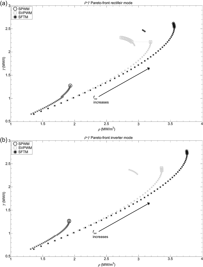
As noted previously for the SPWM, an increase in fsw will improve ρ and γ of the converter with a reduction of the nominal η. However it can be noted, from Figs 9.35 and 9.36, that there is an optimal fsw beyond which ρ or γ will decrease. In the case of VSR with SFTM, the maximum ρ (3.55 MW/m3) and γ (2.62 MW/t) are obtained for the same fsw of 3.79 kHz. In the case of VSI with SFTM, the maximum ρ (3.76 MW/m3) is obtained for fsw = 3.79 kHz, but the maximum γ (2.77 MW/t) is obtained for the maximum possible fsw (4 kHz), which indicates that the IGBT technology limits the maximum γ.
Fig. 9.37 shows the influence of the modulation method on the η–ρ Pareto-front for VSR (Fig. 9.37(a)) and VSI (Fig. 9.37(b)). It is clear that SFTM will give the best trade-off between η and ρ, and only comparable solutions are obtained with SVPWM for small values of fsw, which imply low ρ.
The ρ–γ Pareto-front of 2L-VSC with the three modulation strategies is shown in Fig 9.38(a,b) for VSR and VSI, respectively. Again, SFTM presents the best trade-off between ρ and γ, where the Pareto-front is obtained for the solution with the highest switching frequencies.


9.6.3. Optimal selection of the switching frequency in a 2L-VSC
From Figs 9.35 and 9.36, it can be noted that η decreases with fsw, but there is one fsw that maximizes ρ (or also γ). Then an optimal fsw can be obtained for a given set of system parameters and design constraints. The criterion to select fsw can be to maximize the following objective function:
![]() [9.98]
[9.98]
where ηmax, ρmax and γmax are the maximum values of nominal η, ρ and γ, respectively, for a set of design parameters and constraints. Fig. 9.39 shows the objective function as a function of fsw for the design example 1-MW 2L-VSC with SVPWM (on top) and SFTM (on the bottom) for each operative mode (VSR or VSI). Table 9.8 presents the results of the performance indices when fsw is selected to maximize Eq. [9.98].
Finally, an optimized design of a 2L-VSR is done for different converter nominal power and the parameters and constraint presented in Table 9.7. It is assumed that 2L-VSR is interfacing a wind power generator with an equivalent generator inductance per phase of 1e-4 = 10−4 = 0.0001 in per unit, which is assumed to be the same value for all the nominal power. This low inductance value has been chosen in order to acquire higher inductance values in the input filter and therefore see how the performance indices are affected when the switching frequency is changed.

Figure 9.39 Objective function as function of switching frequency for the design example 1-MW 690-V 2L-VSC: (a) SVPWM; (b) SFTM.
Table 9.8
Results of the optimal selection of switching frequency follows the objective function (Eq. [9.98]) for the 1-MW 2L-VSC
| Modulation | Operation mode | Switching freq. [kHz] | Nominal efficiency [%] | Power density [MW/m3] | Power to mass ratio [MW/t] | Objective function value |
| SVPWM | VSR | 3.107 | 93.68 | 2.938 | 2.141 | 2.927 |
| VSI | 3.437 | 94.22 | 3.36 | 2.409 | 2.956 | |
| SFTM | VSR | 3.807 | 94.01 | 3.547 | 2.615 | 2.950 |
| VSI | 4.000 | 93.64 | 3.754 | 2.773 | 2.950 |

Fig. 9.40 shows the results of the optimized selection of fsw as a function of PN when SVPWM is selected for 2L-VSR. Fig. 9.40(a) shows the selecting of fsw based on four criteria to maximize η, ρ, γ or Λ. Fig. 9.40(b) presents the number of IGBT modules in parallel connection needed when fsw is selected to maximize Λ.
The nominal η, ρ and γ, as functions of the nominal power, are shown in Fig 9.40(c,d,e), respectively. Each of these figures includes the maximum possible value (by selection of the corresponding fsw in Fig. 9.40(a)) and the value obtained when fsw is selected to maximize Λ.
The results of the optimized selection of fsw as function of PN when SFTM is selected for 2L-VSR are shown in Fig. 9.41. Since SFTM is more efficient than SVPWM for the given power factor (0.85), then higher fsw can be used for SFTM and therefore higher ρ and γ are obtained with the same nominal η.


..................Content has been hidden....................
You can't read the all page of ebook, please click here login for view all page.