

108 EMPIRICAL RESULTS
0
20
40
60
80
100
NYSE (O) NYSE (N) TSE SP500 MSCI DJIA
Volatility risk (%)
Datasets
Market
BCRP
Anticor
Β
ΝΝ
CORN
PAMR
CWMR
OLMAR
(a)
0
20
40
60
80
100
NYSE (O) NYSE (N) TSE SP500 MSCI DJIA
MDD risk (%)
Datasets
Market
BCRP
Anticor
Β
ΝΝ
CORN
PAMR
CWMR
OLMAR
(b)
0
5
10
NYSE (O) NYSE (N) TSE SP500 MSCI DJIA
Sharpe ratio
Datasets
Market
BCRP
Anticor
Β
ΝΝ
CORN
PAMR
CWMR
OLMAR
(c)
0
5
10
NYSE (O) NYSE (N) TSE SP500 MSCI DJIA
Calmar ratio
Datasets
Market
BCRP
Anticor
Β
ΝΝ
CORN
PAMR
CWMR
OLMAR
(d)
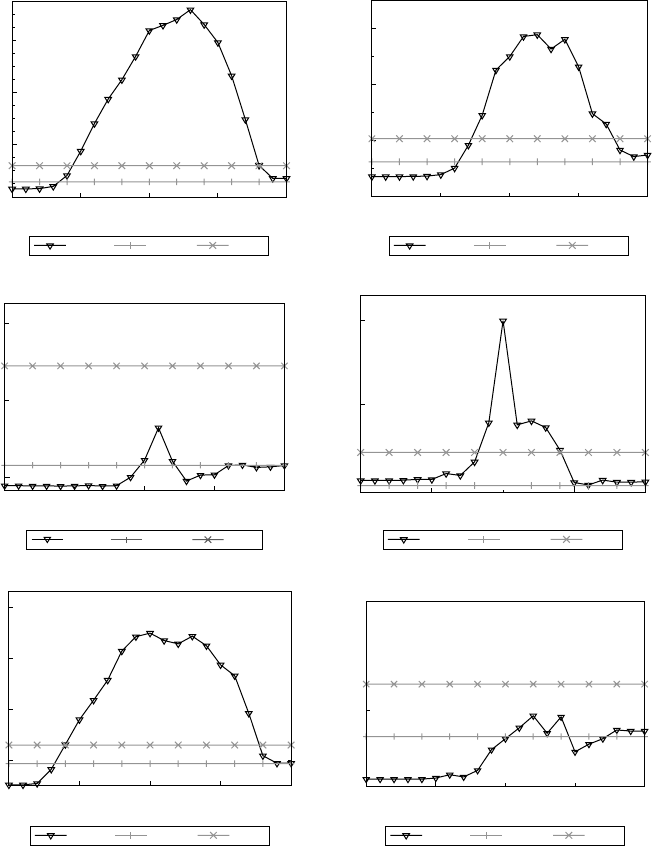
Figure 13.2 Risk and risk-adjusted performance of various strategies on the six datasets.
In each diagram, the rightmost four bars represent the results of our proposed strategies:
(a) volatility risk; (b) drawdown risk; (c) Sharpe ratio; and (d) Calmar ratio.
without high risk.
∗
The volatility risk in Figure 13.2a shows that the proposed four
methods almost achieve the highest risk in terms of volatility risk on most datasets. On
the other hand, the drawdown risk in Figure 13.2b shows that the proposed methods
also achieve high drawdown risk in most datasets. These results validate the notion
that high return is often associated with high risk.
To further evaluate the return and risk, we examine the risk-adjusted return in
terms of an annualized SR and CR. The results in Figure 13.2c and 13.2d clearly
show that CORN, PAMR, and CWMR achieve excellent performance in most cases,
∗
It is true for the long-only portfolio, which is our setting. However, such a statement may be suspect
in regard to long-short portfolios.
T&F Cat #K23731 — K23731_C013 — page 108 — 9/28/2015 — 21:35
EXPERIMENT 3 109
except the DJIAdataset; and OLMAR achieves excellent performance in all datasets.
These encouraging results show that the proposed methods are able to reach a good
trade-off between return and risk, even though we do not explicitly consider risk in
the method formulations.
∗
13.3 Experiment 3: Evaluation of Parameter Sensitivity
In the following four subsections, we evaluate how different choices of parameters
affect the proposed four strategies.
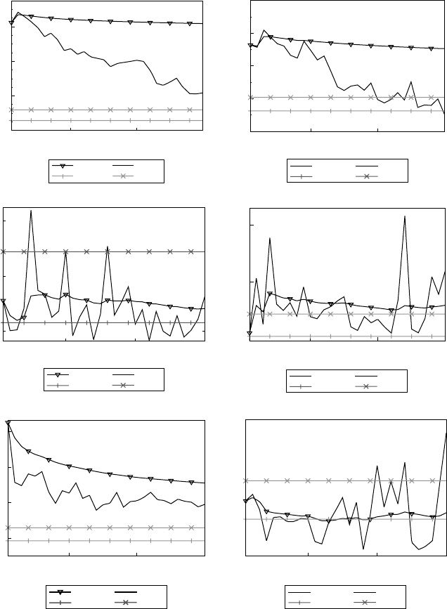
13.3.1 CORN’s Parameter Sensitivity
The proposed CORN has two parameters, that is, the correlation coefficient thres-
hold ρ and the window size for the experts w (or W ).
First, let us see the effects of ρ with fixed W , in Figure 13.3. Clearly, the figures
validate the preliminary analysis in Section 8.4. In general, CORN achieves the best
performance when ρ is around 0, as the figures often peak around 0 or some small
positive values; and, when ρ approaches −1 or 1, CORN’s performance degrades.
Although CORN does not perform well on the TSE and DJIA datasets, on which the
cumulative wealth is often less than the BCRP strategy, it significantly outperforms
the two benchmarks on other datasets. Based on the above observation, choosing a
satisfying ρ for CORN is straightforward, as some small positive values often give
good performance on all datasets.
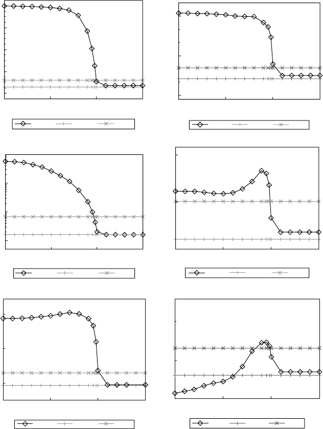
We also examine the effects of W with fixed ρ in Figure 13.4. Note that here CORN
denotes the CORN experts with a specified w and CORN-U denotes the uniform com-
bination of CORN experts with w from 1 to W . Although the cumulative wealth
achieved by CORN experts fluctuates with different w’s, CORN-U’s cumulative
wealth is much more robust with respect to W . Such an observation validates the
effectiveness of the proposed CORN-U and eases the selection of a satisfying W.
13.3.2 PAMR’s Parameter Sensitivity
In this section, we examine PAMR’s parameters, that is, the mean reversion threshold
for the three algorithms and the aggressiveness parameter C for the two variants.
First, we examine the effect of on PAMR’s cumulative wealth. As is greater
than 1, PAMR degrades to uniform constant rebalanced portfolios (CRP) strategy, and
the wealth stabilizes at a constant value achieved by uniform CRP. Thus, we show the
effect of in the range of [0, 1.5]. Figure 13.5 shows the cumulative wealth achieved
by PAMR with varying and two benchmarks, that is, Market and BCRP. Results on
most datasets, except the DJIA dataset, show that the cumulative wealth achieved by
PAMR consistently grows as approaches 0. That is, the smaller the threshold, the
higher the cumulative wealth is, which validates that the motivating mean reversion
does exist on most stock markets. Moreover, in most cases, the cumulative wealth
tends to stabilize as crosses certain dataset-dependent thresholds. As stated before,
∗
We will study it in future.
T&F Cat #K23731 — K23731_C013 — page 109 — 9/28/2015 — 21:35
110 EMPIRICAL RESULTS
10
0
10
4
10
8
10
12
–1 –0.5 0 0.5 1
Total wealth achieved
ρ
(a)
CORN
Market
BCRP
10
0
10
2
10
4
10
6
–1 –0.5 0 0.5 1
Total wealth achieved
ρ
(b)
CORN
Market
BCRP
1
5
9
–1 –0.5 0
(c)
0.5 1
Total wealth achieved
ρ
CORN
Market
BCRP
1
8
15
–1 –0.5 0 0.5 1
Total wealth achieved
ρ
(d)
CORN
Market
BCRP
1
4
16
64
–1 –0.5 0 0.5 1
Total wealth achieved
ρ
(e)
CORN Market
BCRP
1
2
–1 –0.5
(f)
0.501
Total wealth achieved
ρ
CORN
Market
BCRP
Figure 13.3 Parameter sensitivity of CORN-U with respect to ρ with fixed W (W = 5):
(a) NYSE (O); (b) NYSE (N); (c) TSE; (d) SP500; (e) MSCI; and (f) DJIA.
we choose = 0.5 in the experiments, with which the cumulative wealth stabilizes
in most cases. Contrarily, on the DJIA dataset, as approaches 0, the cumulative
wealth achieved by PAMR drops. Such phenomena can be interpreted to mean that
the motivating (single-period) mean reversion does not exist on the dataset, at least in
T&F Cat #K23731 — K23731_C013 — page 110 — 9/28/2015 — 21:35
EXPERIMENT 3 111
10
0
10
4
10
8
10
12
1
10
(a)
20 30
Total wealth achieved
W
CORN-U CORN
Market
BCRP
10
0
10
2
10
4
10
6
1 10 20 30
Total wealth achieved
W
(b)
CORNCORN-U
Market
BCRP
1
5
9
1
10 20 30
Total wealth achieved
W
(c)
CORNCORN-U
Market
BCRP
1
8
15
110 20 30
Total wealth achieved
W
(d)
CORNCORN-U
Market
BCRP
1
4
16
64
110 20 30
Total wealth achieved
W
(e)
CORNCORN-U
Market
BCRP
1
2
110 20 30
Total wealth achieved
W
(f)
CORNCORN-U
Market
BCRP
Figure 13.4 Parameter sensitivity of CORN-U with respect to w (W) with fixed ρ (ρ = 0.1):
(a) NYSE (O); (b) NYSE (N); (c) TSE; (d) SP500; (e) MSCI; and (f) DJIA.
the sense of our motivation. We also note that, on some datasets, PAMR with = 0
achieves the best. Though = 0 means moving more weights to underperforming
stocks, it may not mean moving everything to the worst stock. On the one hand, the
objectives in the formulations would prevent the next portfolio from being far from the
T&F Cat #K23731 — K23731_C013 — page 111 — 9/28/2015 — 21:35
112 EMPIRICAL RESULTS
10
0
10
4
10
8
10
12
10
16
0
ε
(a)
0.5 1 1.5
Total wealth achieved
PAMR
Market BCRP
10
0
10
3
10
6
0
(b)
0.5 1 1.5
Total wealth achieved
ε
PAMR
Market BCRP
10
0
10
1
10
2
10
3
0
(c)
0.5 1 1.5
Total wealth achieved
ε
PAMR Market
BCRP
1
4
16
0
(d)
0.5 1 1.5
Total wealth achieved
ε
PAMR
Market
BCRP
1
4
16
0 0.5
(e)
ε
1 1.5
Total wealth achieved
PAMR
Market BCRP
1
3
00.5
(f)
1 1.5
Total wealth achieved
ε
PAMR
BCRP
Market
Figure 13.5 Parameter sensitivity of PAMR with respect to : (a) NYSE (O); (b) NYSE (N);
(c) TSE; (d) SP500; (e) MSCI; and (f) DJIA.
last portfolio. On the other hand, PAMR-1 and PAMR-2 are designed to alleviate the
huge changes. In summary, the experimental results indicate that the proposed PAMR
is robust with respect to the mean reversion sensitivity parameter, in most cases.
Second, we evaluate the other important parameter for both PAMR-1 and
PAMR-2, that is, the aggressiveness parameter C. Figure 13.6 shows the effects on the
T&F Cat #K23731 — K23731_C013 — page 112 — 9/28/2015 — 21:35
..................Content has been hidden....................
You can't read the all page of ebook, please click here login for view all page.