
12
Dates and Times
One of the bigger reasons for using Pandas is its ability to work with timeseries data. We observed some of this capability earlier, when we concatenated data in Chapter 6 and saw how the indices automatically aligned themselves. This chapter focuses on the more common tasks encountered when working with data that involve dates and times.
Learning Objectives
Create date objects with the
datetimelibraryUse functions to convert strings into a date
Use functions to format dates
Perform date calculations
Use functions to resample dates
Use functions to work with and convert time zones
12.1 Python's datetime Object
Python has a built-in datetime object that is found in the datetime library.
from datetime import datetimeWe can use datetime to get the current date and time.
now = datetime.now()
print(f"Last time this chapter was rendered for print: {now}")
Last time this chapter was rendered for print: 2022-09-01 01:55:41.496795We can also create our own datetime manually.
t1 = datetime.now()
t2 = datetime(1970, 1,1)
And we can do datetime math.
diff = t1 - t2
print(diff)
19236 days, 1:55:41.499914The data type of a date calculation is a timedelta.
print(type(diff))<class 'datetime.timedelta'>We can perform these types of actions when working within a Pandas dataframe.
12.2 Converting to datetime
Converting an object type into a datetime type is done with the to_datatime function. Let’s load up our Ebola data set and convert the Date column into a proper datetime object.
import pandas as pd
ebola = pd.read_csv('data/country_timeseries.csv')

# top left corner of the data
print(ebola.iloc[:5, :5])
Date Day Cases_Guinea Cases_Liberia Cases_SierraLeone
0 1/5/2015 289 2776.0 NaN 10030.0
1 1/4/2015 288 2775.0 NaN 9780.0
2 1/3/2015 287 2769.0 8166.0 9722.0
3 1/2/2015 286 NaN 8157.0 NaN
4 12/31/2014 284 2730.0 8115.0 9633.0The first Date column contains date information, but the .info() attribute tells us it is actually encoded as a generic string object in Pandas.
print(ebola.info())<class 'pandas.core.frame.DataFrame'>
RangeIndex: 122 entries, 0 to 121
Data columns (total 18 columns):
# Column Non-Null Count Dtype
--- ------ -------------- -----
0 Date 122 non-null object
1 Day 122 non-null int64
2 Cases_Guinea 93 non-null float64
3 Cases_Liberia 83 non-null float64
4 Cases_SierraLeone 87 non-null float64
5 Cases_Nigeria 38 non-null float64
6 Cases_Senegal 25 non-null float64
7 Cases_UnitedStates 18 non-null float64
8 Cases_Spain 16 non-null float64
9 Cases_Mali 12 non-null float64
10 Deaths_Guinea 92 non-null float64
11 Deaths_Liberia 81 non-null float64
12 Deaths_SierraLeone 87 non-null float64
13 Deaths_Nigeria 38 non-null float64
14 Deaths_Senegal 22 non-null float64
15 Deaths_UnitedStates 18 non-null float64
16 Deaths_Spain 16 non-null float64
17 Deaths_Mali 12 non-null float64
dtypes: float64(16), int64(1), object(1)
memory usage: 17.3+ KB
NoneWe can create a new column, date_dt, that converts the Date column into a datetime.
ebola['date_dt'] = pd.to_datetime(ebola['Date'])We can also be a little more explicit with how we convert data into a datetime object.
The to_datetime() function has a parameter called format that allows you to manually specify the format of the date you are hoping to parse. Since our date is in a month/day/year format, we can pass in the string %m/%d/%Y.
ebola['date_dt'] = pd.to_datetime(ebola['Date'], format='%m/%d/%Y')In both cases, we end up with a new column with a datetime type.
print(ebola.info())<class 'pandas.core.frame.DataFrame'>
RangeIndex: 122 entries, 0 to 121
Data columns (total 21 columns):
# Column Non-Null Count Dtype
--- ------ -------------- -----
0 Date 122 non-null object
1 Day 122 non-null int64
2 Cases_Guinea 93 non-null float64
3 Cases_Liberia 83 non-null float64
4 Cases_SierraLeone 87 non-null float64
5 Cases_Nigeria 38 non-null float64
6 Cases_Senegal 25 non-null float64
7 Cases_UnitedStates 18 non-null float64
8 Cases_Spain 16 non-null float64
9 Cases_Mali 12 non-null float64
10 Deaths_Guinea 92 non-null float64
11 Deaths_Liberia 81 non-null float64
12 Deaths_SierraLeone 87 non-null float64
13 Deaths_Nigeria 38 non-null float64
14 Deaths_Senegal 22 non-null float64
15 Deaths_UnitedStates 18 non-null float64
16 Deaths_Spain 16 non-null float64
17 Deaths_Mali 12 non-null float64
18 date_dt 122 non-null datetime64[ns]
19 date_dt_a 122 non-null datetime64[ns]
20 date_dt_al 122 non-null datetime64[ns]
dtypes: datetime64[ns](3), float64(16), int64(1), object(1)
memory usage: 20.1+ KB
NoneThe to_datetime() function includes convenient built-in options. For example, you can set the dayfirst or yearfirst options to True if the date format begins with a day (e.g., 31-03-2014) or if the date begins with a year (e.g., 2014-03-31), respectively.
For other date formats, you can manually specify how they are represented using the syntax specified by python’s strptime.1 This syntax is replicated in Table 12.1 from the official Python documentation.
1. strftime (string format time) and strptime (string parse time) behavior: https://docs.python.org/3/library/datetime.html#strftime-and-strptime-behavior
Table 12.1 Python strftime and strptime Behavior (reproduced from the official Python documentation2)
Directive | Meaning | Example | |
|---|---|---|---|
%a | Weekday abbreviated name | Sun, Mon, …, Sat | |
%A | Weekday full name | Sunday, Monday, …, Saturday | |
%w | Weekday as a number, where 0 is Sunday | 0, 1, …, 6 | |
%d | Day of the month as a two-digit number | 01, 02, …, 31 | |
%b | Month abbreviated name | Jan, Feb, …, Dec | |
%B | Month full name | January, February, …, December | |
%m | Month as a two-digit number | 01, 02, …, 12 | |
%y | Year as a two-digit number | 00, 01, …, 99 | |
%Y | Year as a four-digit number | 0001, 0002, …, 2013, 2014, …, 9999 | |
%H | Hour (24-hour clock) as a two-digit number | 00, 01, …, 23 | |
%I | Hour (12-hour clock) as a two-digit number | 01, 02, …, 12 | |
%p | AM or PM | AM, PM | |
%M | Minute as a two-digit number | 00, 01, …, 59 | |
%S | Second as a two-digit number | 00, 01, …, 59 | |
%f | Microsecond as a number | 000000, 000001, …, 999999 | |
%z | UTC offset in the form of +HHMM or hbox{--HHMM} | (empty), +0000, -0400, +1030 | |
%Z | Time zone name | (empty), UTC, EST, CST | |
%j | Day of the year as a three-digit number | 001, 002, …, 366 | |
%U | Week number of the year (Sunday first) | 00, 01, …, 53 | |
%W | Week number of the year (Monday first) | 00, 01, …, 53 | |
%c | Date and time representation | Tue Aug 16 21:30:00 1988 |
|
%x | Date representation | 08/16/88 (None);08/16/1988 |
|
%X | Time representation | 21:30:00 | |
%% | Literal % character | % | |
%G | ISO 8601 year | 0001, 0002, …, 2013, 2014, …, 9999 | |
%u | ISO 8601 weekday | 1, 2, …, 7 | |
%V | ISO 8601 week | 01, 02, …, 53 |
2. strftime (string format time) and strptime (string parse time) behavior: https://docs.python.org/3/library/datetime.html#strftime-and-strptime-behavior
12.3 Loading Data That Include Dates
Many of the data sets used in this book are in a CSV format, or else they come from the seaborn library. The gapminder data set was an exception: It was a tab-separated file (TSV). The read_csv() function has a lot of parameters – for example, parse_dates, inher_datetime_format, keep_date_col, date_parser, dayfirst, and cache_dates. We can parse the Date column directly by specifying the column we want in the parse_dates parameter.
ebola = pd.read_csv('data/country_timeseries.csv', parse_dates=["Date"])
print(ebola.info())
<class 'pandas.core.frame.DataFrame'>
RangeIndex: 122 entries, 0 to 121
Data columns (total 18 columns):
# Column Non-Null Count Dtype
--- ------ -------------- -----
0 Date 122 non-null datetime64[ns]
1 Day 122 non-null int64
2 Cases_Guinea 93 non-null float64
3 Cases_Liberia 83 non-null float64
4 Cases_SierraLeone 87 non-null float64
5 Cases_Nigeria 38 non-null float64
6 Cases_Senegal 25 non-null float64
7 Cases_UnitedStates 18 non-null float64
8 Cases_Spain 16 non-null float64
9 Cases_Mali 12 non-null float64
10 Deaths_Guinea 92 non-null float64
11 Deaths_Liberia 81 non-null float64
12 Deaths_SierraLeone 87 non-null float64
13 Deaths_Nigeria 38 non-null float64
14 Deaths_Senegal 22 non-null float64
15 Deaths_UnitedStates 18 non-null float64
16 Deaths_Spain 16 non-null float64
17 Deaths_Mali 12 non-null float64
dtypes: datetime64[ns](1), float64(16), int64(1)
memory usage: 17.3 KB
NoneThis example shows how we can automatically convert columns into dates directly when the data are loaded.
12.4 Extracting Date Components
Now that we have a datetime object, we can extract various parts of the date, such as year, month, or day. Here’s an example datetime object.
d = pd.to_datetime('2021-12-14')
print(d)
2021-12-14 00:00:00If we pass in a single string, we get a Timestamp.
print(type(d))<class 'pandas._libs.tslibs.timestamps.Timestamp'>Now that we have a proper datetime, we can access various date components as attributes.
print(d.year)2021print(d.month)12print(d.day)14In Chapter 4, we tidied our data when we needed to parse a column that stored multiple bits of information and used the .str. accessor to use string methods like .split(). We can do something similar here with datetime objects by accessing datetime methods using the .dt. accessor.3 Let’s first re-create our date_dt column.
3. Datetime-like properties: https://pandas.pydata.org/docs/reference/series.html#datetimelike-properties
ebola['date_dt'] = pd.to_datetime(ebola['Date'])We know we can get date components such as the year, month, and day by using the year, month, and day attributes, respectively, on a column basis; we saw how this works when we parsed strings in a column using .str.. Here’s the Date and date_dt columns we just created.
print(ebola[['Date', 'date_dt']]) Date date_dt
0 2015-01-05 2015-01-05
1 2015-01-04 2015-01-04
2 2015-01-03 2015-01-03
3 2015-01-02 2015-01-02
4 2014-12-31 2014-12-31
.. ... ...
117 2014-03-27 2014-03-27
118 2014-03-26 2014-03-26
119 2014-03-25 2014-03-25
120 2014-03-24 2014-03-24
121 2014-03-22 2014-03-22[122 rows x 2 columns]We can create a new year column based on the Date column.
ebola['year'] = ebola['date_dt'].dt.year
print(ebola[['Date', 'date_dt', 'year']])
Date date_dt year
0 2015-01-05 2015-01-05 2015
1 2015-01-04 2015-01-04 2015
2 2015-01-03 2015-01-03 2015
3 2015-01-02 2015-01-02 2015
4 2014-12-31 2014-12-31 2014
.. ... ... ...
117 2014-03-27 2014-03-27 2014
118 2014-03-26 2014-03-26 2014
119 2014-03-25 2014-03-25 2014
120 2014-03-24 2014-03-24 2014
121 2014-03-22 2014-03-22 2014[122 rows x 3 columns]Let’s finish parsing our date.
ebola = ebola.assign(
    month=ebola["date_dt"].dt.month,
    day=ebola["date_dt"].dt.day
)print(ebola[['Date', 'date_dt', 'year', 'month', 'day']]) Date date_dt year month day
0 2015-01-05 2015-01-05 2015 1 5
1 2015-01-04 2015-01-04 2015 1 4
2 2015-01-03 2015-01-03 2015 1 3
3 2015-01-02 2015-01-02 2015 1 2
4 2014-12-31 2014-12-31 2014 12 31
.. ... ... ... ... ...
117 2014-03-27 2014-03-27 2014 3 27
118 2014-03-26 2014-03-26 2014 3 26
119 2014-03-25 2014-03-25 2014 3 25
120 2014-03-24 2014-03-24 2014 3 24
121 2014-03-22 2014-03-22 2014 3 22[122 rows x 5 columns]When we parsed out our dates, the data type was not preserved.
print(ebola.info())<class 'pandas.core.frame.DataFrame'>
RangeIndex: 122 entries, 0 to 121
Data columns (total 22 columns):
# Column Non-Null Count Dtype
--- ------ -------------- -----
0 Date 122 non-null datetime64[ns]
1 Day 122 non-null int64
2 Cases_Guinea 93 non-null float64
3 Cases_Liberia 83 non-null float64
4 Cases_SierraLeone 87 non-null float64
5 Cases_Nigeria 38 non-null float64
6 Cases_Senegal 25 non-null float64
7 Cases_UnitedStates 18 non-null float64
8 Cases_Spain 16 non-null float64
9 Cases_Mali 12 non-null float64
10 Deaths_Guinea 92 non-null float64
11 Deaths_Liberia 81 non-null float64
12 Deaths_SierraLeone 87 non-null float64
13 Deaths_Nigeria 38 non-null float64
14 Deaths_Senegal 22 non-null float64
15 Deaths_UnitedStates 18 non-null float64
16 Deaths_Spain 16 non-null float64
17 Deaths_Mali 12 non-null float64
18 date_dt 122 non-null datetime64[ns]
19 year 122 non-null int64
20 month 122 non-null int64
21 day 122 non-null int64
dtypes: datetime64[ns](2), float64(16), int64(4)
memory usage: 21.1 KB
None12.5 Date Calculations and Timedeltas
One of the benefits of having date objects is being able to do date calculations. Our Ebola data set includes a column named Day that indicates how many days into an Ebola outbreak a country is. We can recreate this column using date arithmetic. Here’s the bottom left corner of our data.
print(ebola.iloc[-5:, :5]) Date Day Cases_Guinea Cases_Liberia Cases_SierraLeone
117 2014-03-27 5 103.0 8.0 6.0
118 2014-03-26 4 86.0 NaN NaN
119 2014-03-25 3 86.0 NaN NaN
120 2014-03-24 2 86.0 NaN NaN
121 2014-03-22 0 49.0 NaN NaNThe first day of the outbreak (the earliest date in this data set) is 2015-03-22. So, if we want to calculate the number of days into the outbreak, we can subtract this date from each date by using the .min() method of the column.
print(ebola['date_dt'].min())2014-03-22 00:00:00We can use this date in our calculation.
ebola['outbreak_d'] = ebola['date_dt'] - ebola['date_dt'].min()print(ebola[['Date', 'Day', 'outbreak_d']]) Date Day outbreak_d
0 2015-01-05 289 289 days
1 2015-01-04 288 288 days
2 2015-01-03 287 287 days
3 2015-01-02 286 286 days
4 2014-12-31 284 284 days
.. ... ... ...
117 2014-03-27 5 5 days
118 2014-03-26 4 4 days
119 2014-03-25 3 3 days
120 2014-03-24 2 2 days
121 2014-03-22 0 0 days[122 rows x 3 columns]When we perform this kind of date calculation, we actually end up with a timedelta object.
print(ebola.info())<class 'pandas.core.frame.DataFrame'>
RangeIndex: 122 entries, 0 to 121
Data columns (total 23 columns):
# Column Non-Null Count Dtype
--- ------ -------------- -----
0 Date 122 non-null datetime64[ns]
1 Day 122 non-null int64
2 Cases_Guinea 93 non-null float64
3 Cases_Liberia 83 non-null float64
4 Cases_SierraLeone 87 non-null float64
5 Cases_Nigeria 38 non-null float64
6 Cases_Senegal 25 non-null float64
7 Cases_UnitedStates 18 non-null float64
8 Cases_Spain 16 non-null float64
9 Cases_Mali 12 non-null float64
10 Deaths_Guinea 92 non-null float64
11 Deaths_Liberia 81 non-null float64
12 Deaths_SierraLeone 87 non-null float64
13 Deaths_Nigeria 38 non-null float64
14 Deaths_Senegal 22 non-null float64
15 Deaths_UnitedStates 18 non-null float64
16 Deaths_Spain 16 non-null float64
17 Deaths_Mali 12 non-null float64
18 date_dt 122 non-null datetime64[ns]
19 year 122 non-null int64
20 month 122 non-null int64
21 day 122 non-null int64
22 outbreak_d 122 non-null timedelta64[ns]
dtypes: datetime64[ns](2), float64(16), int64(4), timedelta64[ns](1)
memory usage: 22.0 KB
NoneWe get timedelta objects as results when we perform calculations with datetime objects.
12.6 Datetime Methods
Let’s look at another data set. This one deals with bank failures.
banks = pd.read_csv('data/banklist.csv')
print(banks.head())
Bank Name
0 Fayette County Bank
1 Guaranty Bank, (d/b/a BestBank in Georgia & Mi...
2 First NBC Bank
3 Proficio Bank
4 Seaway Bank and Trust Company
City ST CERT
0 Saint Elmo IL 1802
1 Milwaukee WI 30003
2 New Orleans LA 58302
3 Cottonwood Heights UT 35495
4 Chicago IL 19328
Acquiring Institution Closing Date Updated Date
0 United Fidelity Bank, fsb 26-May-17 26-Jul-17
1 First-Citizens Bank & Trust Company 5-May-17 26-Jul-17
2 Whitney Bank 28-Apr-17 26-Jul-17
3 Cache Valley Bank 3-Mar-17 18-May-17
4 State Bank of Texas 27-Jan-17 18-May-17Again, we can import our data with the dates directly parsed.
banks = pd.read_csv(
  "data/banklist.csv", parse_dates=["Closing Date", "Updated Date"]
)

print(banks.info())
<class 'pandas.core.frame.DataFrame'>
RangeIndex: 553 entries, 0 to 552
Data columns (total 7 columns):
# Column Non-Null Count Dtype
--- ------ -------------- -----
0 Bank Name 553 non-null object
1 City 553 non-null object
2 ST 553 non-null object
3 CERT 553 non-null int64
4 Acquiring Institution 553 non-null object
5 Closing Date 553 non-null datetime64[ns]
6 Updated Date 553 non-null datetime64[ns]
dtypes: datetime64[ns](2), int64(1), object(4)
memory usage: 30.4+ KB
NoneWe can parse out the date by obtaining the quarter and year in which the bank closed.
banks = banks.assign(
  closing_quarter=banks['Closing Date'].dt.quarter,
  closing_year=banks['Closing Date'].dt.year
)
closing_year = banks.groupby(['closing_year']).size()Alternatively, we can calculate how many banks closed in each quarter of each year.
closing_year_q = (
  banks
  .groupby(['closing_year', 'closing_quarter'])
  .size()
)
We can then plot these results as shown in Figure 12.1 and Figure 12.2.
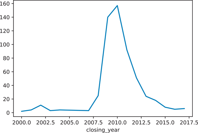
Figure 12.1 Number of banks closing each year
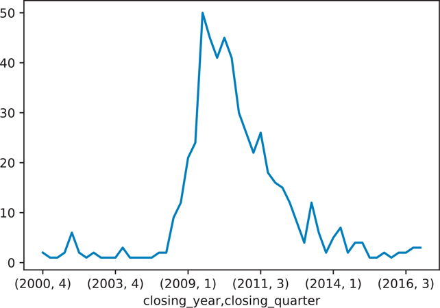
Figure 12.2 Number of banks closing each year by quarter
import matplotlib.pyplot as plt

fig, ax = plt.subplots()
ax = closing_year.plot()
plt.show()
fig, ax = plt.subplots()
ax = closing_year_q.plot()
plt.show()12.7 Getting Stock Data
One commonly encountered type of data that contains dates is stock prices. Luckily Python has a way of getting this type of data programmatically with the pandas-datareader library.4
4. pandas-datareader library: https://pandas-datareader.readthedocs.io/
# we can install and use the pandas_datafreader
# to get data from the Internet
import pandas_datareader.data as web

# in this example we are getting stock information about Tesla
tesla = web.DataReader('TSLA', 'yahoo')

print(tesla)
Date High Low Open Close
2017-09-05 23.699333 23.059334 23.586666 23.306000
2017-09-06 23.398666 22.770666 23.299999 22.968666
2017-09-07 23.498667 22.896667 23.065332 23.374001
2017-09-08 23.318666 22.820000 23.266001 22.893333
2017-09-11 24.247334 23.333332 23.423332 24.246000
... ... ... ... ...
2022-08-25 302.959991 291.600006 302.359985 296.070007
2022-08-26 302.000000 287.470001 297.429993 288.089996
2022-08-29 287.739990 280.700012 282.829987 284.820007
2022-08-30 288.480011 272.649994 287.869995 277.700012
2022-08-31 281.250000 271.809998 280.619995 275.609985 Date Volume Adj Close
2017-09-05 57526500.0 23.306000
2017-09-06 61371000.0 22.968666
2017-09-07 63588000.0 23.374001
2017-09-08 48952500.0 22.893333
2017-09-11 115006500.0 24.246000
... ... ...
2022-08-25 53230000.0 296.070007
2022-08-26 56905800.0 288.089996
2022-08-29 41864700.0 284.820007
2022-08-30 50541800.0 277.700012
2022-08-31 51788900.0 275.609985[1257 rows x 6 columns]# the stock data was saved
# so we do not need to rely on the Internet again
# instead we can load the same data set as a file
tesla = pd.read_csv(
'data/tesla_stock_yahoo.csv', parse_dates=["Date"]
)
print(tesla) Date Open High Low Close
0 2010-06-29 19.000000 25.000000 17.540001 23.889999
1 2010-06-30 25.790001 30.420000 23.299999 23.830000
2 2010-07-01 25.000000 25.920000 20.270000 21.959999
3 2010-07-02 23.000000 23.100000 18.709999 19.200001
4 2010-07-06 20.000000 20.000000 15.830000 16.110001
... ... ... ... ... ...
1786 2017-08-02 318.940002 327.119995 311.220001 325.890015
1787 2017-08-03 345.329987 350.000000 343.149994 347.089996
1788 2017-08-04 347.000000 357.269989 343.299988 356.910004
1789 2017-08-07 357.350006 359.480011 352.750000 355.170013
1790 2017-08-08 357.529999 368.579987 357.399994 365.220001 Adj Close Volume
0 23.889999 18766300
1 23.830000 17187100
2 21.959999 8218800
3 19.200001 5139800
4 16.110001 6866900
... ... ...
1786 325.890015 13091500
1787 347.089996 13535000
1788 356.910004 9198400
1789 355.170013 6276900
1790 365.220001 7449837[1791 rows x 7 columns]12.8 Subsetting Data Based on Dates
Since we now know how to extract parts of a date out of a column (Section 12.4), we can incorporate these methods to subset our data without having to parse out the individual components manually.
For example, if we want only data for June 2010 from our stock price data set, we can use boolean subsetting.
print(
  tesla.loc[
    (tesla.Date.dt.year == 2010) & (tesla.Date.dt.month == 6)
  ]
)
Date Open High Low Close Adj Close
0 2010-06-29 19.000000 25.00 17.540001 23.889999 23.889999
1 2010-06-30 25.790001 30.42 23.299999 23.830000 23.830000 Volume
0 18766300
1 1718710012.8.1 The DatetimeIndex Object
When we are working with datetime data, we often need to set the datetime object to be the dataframe’s index. To this point, we’ve mainly left the dataframe row index to be the row number. We have also seen some side effects that arise because the row index may not always be the row number, such as when we were concatenating dataframes in Chapter 6.
First, let’s assign the Date column as the index.
tesla.index = tesla['Date']
print(tesla.index)
DatetimeIndex(['2010-06-29', '2010-06-30', '2010-07-01',
'2010-07-02', '2010-07-06', '2010-07-07',
'2010-07-08', '2010-07-09', '2010-07-12',
'2010-07-13',
...
'2017-07-26', '2017-07-27', '2017-07-28',
'2017-07-31', '2017-08-01', '2017-08-02',
'2017-08-03', '2017-08-04', '2017-08-07',
'2017-08-08'],
dtype='datetime64[ns]', name='Date', length=1791, freq=None)With the index set as a date object, we can now use the date directly to subset rows. For example, we can subset our data based on the year.
print(tesla['2015']) Date Open High Low
Date
2015-01-02 2015-01-02 222.869995 223.250000 213.259995
2015-01-05 2015-01-05 214.550003 216.500000 207.160004
2015-01-06 2015-01-06 210.059998 214.199997 204.210007
2015-01-07 2015-01-07 213.350006 214.779999 209.779999
2015-01-08 2015-01-08 212.809998 213.800003 210.009995
... ... ... ... ...
2015-12-24 2015-12-24 230.559998 231.880005 228.279999
2015-12-28 2015-12-28 231.490005 231.979996 225.539993
2015-12-29 2015-12-29 230.059998 237.720001 229.550003
2015-12-30 2015-12-30 236.600006 243.630005 235.669998
2015-12-31 2015-12-31 238.509995 243.449997 238.369995 Close Adj Close Volume
Date
2015-01-02 219.309998 219.309998 4764400
2015-01-05 210.089996 210.089996 5368500
2015-01-06 211.279999 211.279999 6261900
2015-01-07 210.949997 210.949997 2968400
2015-01-08 210.619995 210.619995 3442500
... ... ... ...
2015-12-24 230.570007 230.570007 708000
2015-12-28 228.949997 228.949997 1901300
2015-12-29 237.190002 237.190002 2406300
2015-12-30 238.089996 238.089996 3697900
2015-12-31 240.009995 240.009995 2683200[252 rows x 7 columns] print(tesla.loc['2015'])Alternatively, we can subset the data based on the year and month.
print(tesla['2010-06']) Date Open High Low Close
Date
2010-06-29 2010-06-29 19.000000 25.00 17.540001 23.889999
2010-06-30 2010-06-30 25.790001 30.42 23.299999 23.830000 Adj Close Volume
Date
2010-06-29 23.889999 18766300
2010-06-30 23.830000 17187100print(tesla.loc['2010-06'])12.8.2 The TimedeltaIndex Object
Just as we set the index of a dataframe to a datetime to create a DatetimeIndex, so we can do the same thing with a timedelta to create a TimedeltaIndex.
Let’s create a timedelta.
tesla['ref_date'] = tesla['Date'] - tesla['Date'].min()Now we can assign the timedelta to the index.
tesla.index = tesla['ref_date']print(tesla) Date Open High Low
ref_date
0 days 2010-06-29 19.000000 25.000000 17.540001
1 days 2010-06-30 25.790001 30.420000 23.299999
2 days 2010-07-01 25.000000 25.920000 20.270000
3 days 2010-07-02 23.000000 23.100000 18.709999
7 days 2010-07-06 20.000000 20.000000 15.830000
... ... ... ... ...
2591 days 2017-08-02 318.940002 327.119995 311.220001
2592 days 2017-08-03 345.329987 350.000000 343.149994
2593 days 2017-08-04 347.000000 357.269989 343.299988
2596 days 2017-08-07 357.350006 359.480011 352.750000
2597 days 2017-08-08 357.529999 368.579987 357.399994 Close Adj Close Volume ref_date
ref_date
0 days 23.889999 23.889999 18766300 0 days
1 days 23.830000 23.830000 17187100 1 days
2 days 21.959999 21.959999 8218800 2 days
3 days 19.200001 19.200001 5139800 3 days
7 days 16.110001 16.110001 6866900 7 days
... ... ... ... ...
2591 days 325.890015 325.890015 13091500 2591 days
2592 days 347.089996 347.089996 13535000 2592 days
2593 days 356.910004 356.910004 9198400 2593 days
2596 days 355.170013 355.170013 6276900 2596 days
2597 days 365.220001 365.220001 7449837 2597 days[1791 rows x 8 columns]We can now select our data based on these deltas.
print(tesla['0 day': '10 day']) Date Open High Low Close
ref_date
0 days 2010-06-29 19.000000 25.000000 17.540001 23.889999
1 days 2010-06-30 25.790001 30.420000 23.299999 23.830000
2 days 2010-07-01 25.000000 25.920000 20.270000 21.959999
3 days 2010-07-02 23.000000 23.100000 18.709999 19.200001
7 days 2010-07-06 20.000000 20.000000 15.830000 16.110001
8 days 2010-07-07 16.400000 16.629999 14.980000 15.800000
9 days 2010-07-08 16.139999 17.520000 15.570000 17.459999
10 days 2010-07-09 17.580000 17.900000 16.549999 17.400000 Adj Close Volume ref_date
ref_date
0 days 23.889999 18766300 0 days
1 days 23.830000 17187100 1 days
2 days 21.959999 8218800 2 days
3 days 19.200001 5139800 3 days
7 days 16.110001 6866900 7 days
8 days 15.800000 6921700 8 days
9 days 17.459999 7711400 9 days
10 days 17.400000 4050600 10 days12.9 Date Ranges
Not every data set will have a fixed frequency of values. For example, in our Ebola data set, we do not have an observation for every day in the date range.
ebola = pd.read_csv(
'data/country_timeseries.csv', parse_dates=["Date"]
)
Here, 2015-01-01 is missing from the .head() of the data.
print(ebola.iloc[:, :5])
            Date Day  Cases_Guinea  Cases_Liberia  Cases_SierraLeone
0     2015-01-05 289        2776.0            NaN            10030.0
1     2015-01-04 288        2775.0            NaN             9780.0
2     2015-01-03 287        2769.0         8166.0             9722.0
3     2015-01-02 286           NaN         8157.0                NaN
4     2014-12-31 284        2730.0         8115.0             9633.0
..           ... ...           ...            ...                ...
117   2014-03-27   5         103.0            8.0                6.0
118   2014-03-26   4          86.0            NaN                NaN
119   2014-03-25   3          86.0            NaN                NaN
120   2014-03-24   2          86.0            NaN                NaN
121   2014-03-22   0          49.0            NaN                NaN
[122 rows x 5 columns]It’s common practice to create a date range to .reindex() a data set. We can use the date_range()
head_range = pd.date_range(start='2014-12-31', end='2015-01-05')
print(head_range)
DatetimeIndex(['2014-12-31', '2015-01-01', '2015-01-02',
'2015-01-03', '2015-01-04', '2015-01-05'],
dtype='datetime64[ns]', freq='D')We’ll just work with the first five rows in this example.
ebola_5 = ebola.head()If we want to set this date range as the index, we need to first set the date as the index.
ebola_5.index = ebola_5['Date']Next we can .reindex() our data.
ebola_5 = ebola_5.reindex(head_range)

print(ebola_5.iloc[:, :5])
Date Day Cases_Guinea Cases_Liberia
2014-12-31 2014-12-31 284.0 2730.0 8115.0
2015-01-01 NaT NaN NaN NaN
2015-01-02 2015-01-02 286.0 NaN 8157.0
2015-01-03 2015-01-03 287.0 2769.0 8166.0
2015-01-04 2015-01-04 288.0 2775.0 NaN
2015-01-05 2015-01-05 289.0 2776.0 NaN
      Cases_SierraLeone
2014-12-31       9633.0
2015-01-01          NaN
2015-01-02          NaN
2015-01-03       9722.0
2015-01-04       9780.0
2015-01-05      10030.0
12.9.1 Frequencies
When we created our head_range, the print statement included a parameter called freq. In that example, freq was 'D' for “day.” That is, the values in our date range were stepped through using a day-by-day increment. The possible frequencies are reproduced from the Pandas timeseries documentation that is listed in Table 12.2.5
5. Frequency offset aliases: https://pandas.pydata.org/docs/user_guide/timeseries.html#offset-aliases
Table 12.2 Possible Frequencies
|
|
|---|---|
| Business day frequency |
| Custom business day frequency (experimental) |
| Calendar day frequency |
| Weekly frequency |
| Month end frequency |
| Semi-month end frequency (15th and end of month) |
| Business month end frequency |
| Custom business month end frequency |
| Month start frequency |
| Semi-month start frequency (1st and 15th) |
| Business month start frequency |
| Custom business month start frequency |
| Quarter end frequency |
| Business quarter end frequency |
| Quarter start frequency |
| Business quarter start frequency |
| Year end frequency |
| Business year end frequency |
| Year start frequency |
| Business year start frequency |
| Business hour frequency |
| Hour frequency |
| Minute frequency |
| Second frequency |
| Millisecond frequency |
| Microsecond frequency |
| Nanosecond frequency |
These values can be passed into the freq parameter when calling date_range. For example, January 2, 2022, was a Sunday, and we can create a range consisting of the business days in that week.
# business days during the week of Jan 1, 2022
print(pd.date_range('2022-01-01', '2022-01-07', freq='B'))
DatetimeIndex(['2022-01-03', '2022-01-04', '2022-01-05',
'2022-01-06', '2022-01-07'],
dtype='datetime64[ns]', freq='B')12.9.2 Offsets
Offsets are variations on a base frequency. For example, we can take the business days range that we just created and add an offset such that instead of every business day, data are included for every other business day.
# every other business day during the week of Jan 1, 2022
print(pd.date_range('2022-01-01', '2017-01-07', freq='2B'))
DatetimeIndex([], dtype='datetime64[ns]', freq='2B')We created this offset by putting a multiplying value before the base frequency. This kind of offset can be combined with other base frequencies as well. For example, we can specify the first Thursday of each month in the year 2022.
print(pd.date_range('2022-01-01', '2022-12-31', freq='WOM-1THU'))DatetimeIndex(['2022-01-06', '2022-02-03', '2022-03-03',
'2022-04-07', '2022-05-05', '2022-06-02',
'2022-07-07', '2022-08-04', '2022-09-01',
'2022-10-06', '2022-11-03', '2022-12-01'],
dtype='datetime64[ns]', freq='WOM-1THU')We can also specify the third Friday of each month.
print(pd.date_range('2022-01-01', '2022-12-31', freq='WOM-3FRI'))DatetimeIndex(['2022-01-21', '2022-02-18', '2022-03-18',
'2022-04-15', '2022-05-20', '2022-06-17',
'2022-07-15', '2022-08-19', '2022-09-16',
'2022-10-21', '2022-11-18', '2022-12-16'],
dtype='datetime64[ns]', freq='WOM-3FRI')12.10 Shifting Values
There are a few reasons why you might want to shift your dates by a certain value. For example, you might need to correct some kind of measurement error in your data. Alternatively, you might want to standardize the start dates for your data so you can compare trends.
Even though our Ebola data isn’t “tidy,” one of the benefits of the data in its current format is that it allows us to plot the outbreak. This plot is shown in Figure 12.3.
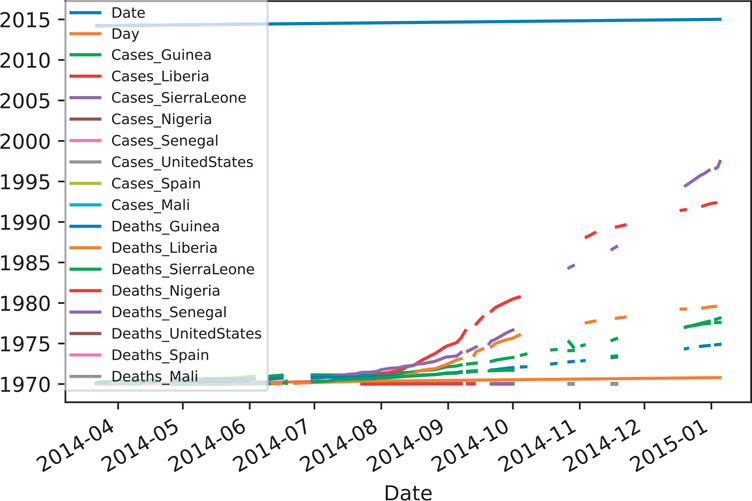
Figure 12.3 Ebola plot of cases and deaths (unshifted dates)
import matplotlib.pyplot as plt

ebola.index = ebola['Date']
fig, ax = plt.subplots()
ax = ebola.plot(ax=ax)
ax.legend(fontsize=7, loc=2, borderaxespad=0.0)
plt.show()When we’re looking at an outbreak, one useful piece of information is how fast an outbreak is spreading relative to other countries. Let’s look at just a few columns from our Ebola data set.
ebola_sub = ebola[['Day', 'Cases_Guinea', 'Cases_Liberia']]
print(ebola_sub.tail(10))
Day Cases_Guinea Cases_Liberia
Date
2014-04-04 13 143.0 18.0
2014-04-01 10 127.0 8.0
2014-03-31 9 122.0 8.0
2014-03-29 7 112.0 7.0
2014-03-28 6 112.0 3.0
2014-03-27 5 103.0 8.0
2014-03-26 4 86.0 NaN
2014-03-25 3 86.0 NaN
2014-03-24 2 86.0 NaN
2014-03-22 0 49.0 NaNYou can see that each country’s starting date is different, which makes it difficult to compare the actual slopes between countries when a new outbreak occurs later in time.
In this example, we want all our dates to start from a common 0 day. There are multiple steps to this process.
Since not every date is listed, we need to create a date range of all the dates in our data set.
We need to calculate the difference between the earliest date in our data set, and the earliest valid (non
NaN) date in each column.We can then shift each of the columns by this calculated value.
Before we begin, let’s start with a fresh copy of the Ebola data set. We’ll parse the Date column as a proper date object, and assign this date to the .index. In this example, we are parsing the date and setting it as the index directly.
ebola = pd.read_csv(
  "data/country_timeseries.csv",
  index_col="Date",
  parse_dates=["Date"],
)

print(ebola.iloc[:, :4])
Day Cases_Guinea Cases_Liberia Cases_SierraLeone
Date
2015-01-05 289 2776.0 NaN 10030.0
2015-01-04 288 2775.0 NaN 9780.0
2015-01-03 287 2769.0 8166.0 9722.0
2015-01-02 286 NaN 8157.0 NaN
2014-12-31 284 2730.0 8115.0 9633.0
... ... ... ... ...
2014-03-27 5 103.0 8.0 6.0
2014-03-26 4 86.0 NaN NaN
2014-03-25 3 86.0 NaN NaN
2014-03-24 2 86.0 NaN NaN
2014-03-22 0 49.0 NaN NaN[122 rows x 4 columns]First, we need to create the date range to fill in all the missing dates in our data. Then, when we shift our date values downward, the number of days that the data will shift will be the same as the number of rows that will be shifted.
new_idx = pd.date_range(ebola.index.min(), ebola.index.max())

print(new_idx)
DatetimeIndex(['2014-03-22', '2014-03-23', '2014-03-24',
'2014-03-25', '2014-03-26', '2014-03-27',
'2014-03-28', '2014-03-29', '2014-03-30',
'2014-03-31',
...
'2014-12-27', '2014-12-28', '2014-12-29',
'2014-12-30', '2014-12-31', '2015-01-01',
'2015-01-02', '2015-01-03', '2015-01-04',
'2015-01-05'],
dtype='datetime64[ns]', length=290, freq='D')Looking at our new_idx, we see that the dates are not in the order that we want. To fix this, we can reverse the order of the index.
new_idx = reversed(new_idx)
print(new_idx)
<reversed object at 0x105aedfc0>Now we can properly .reindex() our data. This will create rows of NaN values if the index does not exist already in our data set.
ebola = ebola.reindex(new_idx)If we look at the .head() and .tail() of the resulting data, we see that dates that were originally not listed have been added into the data set, along with a row of NaN missing values. Additionally, the Date column is filled with the NaT value, which is an internal Pandas representation for missing time value (similar to how NaN is used for numeric missing values).
print(ebola.iloc[:, :4])
             Day Cases_Guinea Cases_Liberia Cases_SierraLeone
Date
2015-01-05  289.0       2776.0           NaN           10030.0
2015-01-04  288.0       2775.0           NaN            9780.0
2015-01-03  287.0       2769.0        8166.0            9722.0
2015-01-02  286.0          NaN        8157.0               NaN
2015-01-01    NaN          NaN           NaN               NaN
...           ...          ...           ...               ...
2014-03-26    4.0         86.0           NaN               NaN
2014-03-25    3.0         86.0           NaN               NaN
2014-03-24    2.0         86.0           NaN               NaN
2014-03-23    NaN          NaN           NaN               NaN
2014-03-22    0.0         49.0           NaN               NaN
[290 rows x 4 columns]Now that we’ve created our date range and assigned it to the index, our next step is to calculate the difference between the earliest date in our data set and the earliest valid (non-missing) date in each column. To perform this calculation, we can use the Series method called .last_valid_index(), which returns the label (index) of the last non-missing or non-null value. An analogous method called .first_valid_index() returns the first non-missing or non-null value. Since we want to perform this calculation across all the columns, we can use the .apply() method.
last_valid = ebola.apply(pd.Series.last_valid_index)
print(last_valid)
Day 2014-03-22
Cases_Guinea 2014-03-22
Cases_Liberia 2014-03-27
Cases_SierraLeone 2014-03-27
Cases_Nigeria 2014-07-23
...
Deaths_Nigeria 2014-07-23
Deaths_Senegal 2014-09-07
Deaths_UnitedStates 2014-10-01
Deaths_Spain 2014-10-08
Deaths_Mali 2014-10-22
Length: 17, dtype: datetime64[ns]Next, we want to get the earliest date in our data set.
earliest_date = ebola.index.min()
print(earliest_date)
2014-03-22 00:00:00We then subtract this date from each of our last_valid dates.
shift_values = last_valid - earliest_date
print(shift_values)
Day 0 days
Cases_Guinea 0 days
Cases_Liberia 5 days
Cases_SierraLeone 5 days
Cases_Nigeria 123 days
...
Deaths_Nigeria 123 days
Deaths_Senegal 169 days
Deaths_UnitedStates 193 days
Deaths_Spain 200 days
Deaths_Mali 214 days
Length: 17, dtype: timedelta64[ns]Finally, we can iterate through each column, using the .shift() method to shift the columns down by the corresponding value in shift_values. Note that the values in shift_values are all positive. If they were negative (if we flipped the order of our subtraction), this operation would shift the values up.
ebola_dict = {}

for idx, col in enumerate(ebola):
    d = shift_values[idx].days
    shifted = ebola[col].shift(d)
    ebola_dict[col] = shifted

#print(ebola_dict)
Since we have a dict of values, we can convert it to a dataframe using the Pandas DataFrame function.
ebola_shift = pd.DataFrame(ebola_dict)The last row in each column now has a value; that is, the columns have been shifted down appropriately.
print(ebola_shift.tail()) Day Cases_Guinea Cases_Liberia Cases_SierraLeone
Date
2014-03-26 4.0 86.0 8.0 2.0
2014-03-25 3.0 86.0 NaN NaN
2014-03-24 2.0 86.0 7.0 NaN
2014-03-23 NaN NaN 3.0 2.0
2014-03-22 0.0 49.0 8.0 6.0
           Cases_Nigeria Cases_Senegal  Cases_UnitedStates
Date
2014-03-26           1.0           NaN                1.0
2014-03-25           NaN           NaN                NaN
2014-03-24           NaN           NaN                NaN
2014-03-23           NaN           NaN                NaN
2014-03-22           0.0           1.0                1.0
Cases_Spain Cases_Mali Deaths_Guinea Deaths_Liberia
Date
2014-03-26 1.0 NaN 62.0 4.0
2014-03-25 NaN NaN 60.0 NaN
2014-03-24 NaN NaN 59.0 2.0
2014-03-23 NaN NaN NaN 3.0
2014-03-22 1.0 1.0 29.0 6.0 Deaths_SierraLeone Deaths_Nigeria Deaths_Senegal
Date
2014-03-26 2.0 1.0 NaN
2014-03-25 NaN NaN NaN
2014-03-24 NaN NaN NaN
2014-03-23 2.0 NaN NaN
2014-03-22 5.0 0.0 0.0 Deaths_UnitedStates Deaths_Spain Deaths_Mali
Date
2014-03-26 0.0 1.0 NaN
2014-03-25 NaN NaN NaN
2014-03-24 NaN NaN NaN
2014-03-23 NaN NaN NaN
2014-03-22 0.0 1.0 1.0Finally, since the indices are no longer valid across each row, we can remove them, and then assign the correct index, which is the Day. Note that Day no longer represents the first day of the entire outbreak, but rather the first day of an outbreak for the given country.
ebola_shift.index = ebola_shift['Day']
ebola_shift = ebola_shift.drop(['Day'], axis="columns")
print(ebola_shift.tail())
      Cases_Guinea Cases_Liberia Cases_SierraLeone Cases_Nigeria
Day
4.0           86.0           8.0               2.0           1.0
3.0           86.0           NaN               NaN           NaN
2.0           86.0           7.0               NaN           NaN
NaN            NaN           3.0               2.0           NaN
0.0           49.0           8.0               6.0           0.0
Cases_Senegal Cases_UnitedStates Cases_Spain Cases_Mali
Day
4.0 NaN 1.0 1.0 NaN
3.0 NaN NaN NaN NaN
2.0 NaN NaN NaN NaN
NaN NaN NaN NaN NaN
0.0 1.0 1.0 1.0 1.0 Deaths_Guinea Deaths_Liberia Deaths_SierraLeone
Day
4.0 62.0 4.0 2.0
3.0 60.0 NaN NaN
2.0 59.0 2.0 NaN
NaN NaN 3.0 2.0
0.0 29.0 6.0 5.0 Deaths_Nigeria Deaths_Senegal Deaths_UnitedStates
Day
4.0 1.0 NaN 0.0
3.0 NaN NaN NaN
2.0 NaN NaN NaN
NaN NaN NaN NaN
0.0 0.0 0.0 0.0 Deaths_Spain Deaths_Mali
Day
4.0 1.0 NaN
3.0 NaN NaN
2.0 NaN NaN
NaN NaN NaN
0.0 1.0 1.012.11 Resampling
Resampling converts a datetime from one frequency to another frequency. Three types of resampling can occur:
Downsampling: from a higher frequency to a lower frequency (e.g., daily to monthly)
Upsampling: from a lower frequency to a higher frequency (e.g., monthly to daily)
No change: frequency does not change (e.g., every first Thursday of the month to the last Friday of the month)
The values we can pass into .resample() are listed in Table 12.2.
# downsample daily values to monthly values
# since we have multiple values, we need to aggregate the results
# here we will use the mean
down = ebola.resample('M').mean()
print(down.iloc[:,  :5])
Day Cases_Guinea Cases_Liberia
Date
2014-03-31 4.500000 94.500000 6.500000
2014-04-30 24.333333 177.818182 24.555556
2014-05-31 51.888889 248.777778 12.555556
2014-06-30 84.636364 373.428571 35.500000
2014-07-31 115.700000 423.000000 212.300000
... ... ... ...
2014-09-30 177.500000 967.888889 2815.625000
2014-10-31 207.470588 1500.444444 4758.750000
2014-11-30 237.214286 1950.500000 7039.000000
2014-12-31 271.181818 2579.625000 7902.571429
2015-01-31 287.500000 2773.333333 8161.500000 Cases_SierraLeone Cases_Nigeria
Date
2014-03-31 3.333333 NaN
2014-04-30 2.200000 NaN
2014-05-31 7.333333 NaN
2014-06-30 125.571429 NaN
2014-07-31 420.500000 1.333333
... ... ...
2014-09-30 1726.000000 20.714286
2014-10-31 3668.111111 20.000000
2014-11-30 5843.625000 20.000000
2014-12-31 8985.875000 20.000000
2015-01-31 9844.000000 NaN[11 rows x 5 columns]# here we will upsample our downsampled value
# notice how missing dates are populated,
# but they are filled in with missing values
up = down.resample('D').mean()
print(up.iloc[:, :5]) Day Cases_Guinea Cases_Liberia Cases_SierraLeone
Date
2014-03-31 4.5 94.500000 6.5 3.333333
2014-04-01 NaN NaN NaN NaN
2014-04-02 NaN NaN NaN NaN
2014-04-03 NaN NaN NaN NaN
2014-04-04 NaN NaN NaN NaN
... ... ... ... ...
2015-01-27 NaN NaN NaN NaN
2015-01-28 NaN NaN NaN NaN
2015-01-29 NaN NaN NaN NaN
2015-01-30 NaN NaN NaN NaN
2015-01-31 287.5 2773.333333 8161.5 9844.000000 Cases_Nigeria
Date
2014-03-31 NaN
2014-04-01 NaN
2014-04-02 NaN
2014-04-03 NaN
2014-04-04 NaN
... ...
2015-01-27 NaN
2015-01-28 NaN
2015-01-29 NaN
2015-01-30 NaN
2015-01-31 NaN[307 rows x 5 columns]12.12 Time Zones
Don’t try to write your own time zone converter. As Tom Scott explains in a “Computerphile” video, “That way lies madness.”6 There are many things you probably did not even think to consider when working with different time zones. For example, not every country implements daylight savings time, and even those that do, may not necessarily change the clocks on the same day of the year. And don’t forget about leap years and leap seconds! Luckily Python has a library specifically designed to work with time zones7, Pandas also wraps this library when working with time zones.
6. The problem with time and time zones: Computerphile: www.youtube.com/watch?v=-5wpm-gesOY
7. Documentation for pytz:a https://pythonhosted.org/pytz/
import pytzThere are many time zones available in the library.
print(len(pytz.all_timezones))594Here are the U.S. time zones:
import re
regex = re.compile(r'^US')
selected_files = filter(regex.search, pytz.common_timezones)
print(list(selected_files))
['US/Alaska', 'US/Arizona', 'US/Central', 'US/Eastern', 'US/Hawaii',
' US/Mountain', 'US/Pacific']The easiest way to interact with time zones in Pandas is to use the string names given in pytz.all_timezones().
One way to illustrate time zones is to create two timestamps using the Pandas Timestamp function. For example, if there was a flight between the JFK and LAX airports that departed at 7:00 AM from New York and landed at 9:57 AM in Los Angeles. We can encode these times with the proper time zone.
# 7AM Eastern
depart = pd.Timestamp('2017-08-29 07:00', tz='US/Eastern')
print(depart)
2017-08-29 07:00:00-04:00arrive = pd.Timestamp('2017-08-29 09:57')
print(arrive)2017-08-29 09:57:00Another way we can encode a time zone is by using the .tz_localize() method on an “empty” timestamp.
arrive = arrive.tz_localize('US/Pacific')
print(arrive)
2017-08-29 09:57:00-07:00We can convert the arrival time back to the Eastern time zone to see what the time would be on the East Coast when the flight arrives.
print(arrive.tz_convert('US/Eastern'))2017-08-29 12:57:00-04:00We can also perform operations on time zones. Here we look at the difference between the times to get the flight duration.
duration = arrive - depart
print(duration)
0 days 05:57:0012.13 Arrow for Better Dates and Times
If you do end up working with date and time columns often, I would suggest looking into the arrow library. You can find the documentation page here: https://arrow.readthedocs.io/en/latest/ Do not confuse this Arrow library with the Apache Arrow project for language-independent dataframe formats.
Arrow is a separate library that needs to be installed, but works slightly different from the methods shown in this chapter. However, it does do a better job handling time zones. See this post by Paul Ganssle for more information about the benefits of arrow over pytz: https://blog.ganssle.io/articles/2018/03/pytz-fastest-footgun.html
Conclusion
Pandas provides a series of convenient methods and functions when we are working with dates and times because these types of data are used so often with time-series data. A common example of time-series data is stock prices, but other examples include observational and simulated data. These convenient Pandas functions and methods allow you to easily work with date objects without having to resort to string manipulation and parsing.