Search in book...
Toggle Font Controls
Create new playlist

Name your new playlist

Playlist description (optional)
Sign In

Email address

Password

Forgot Password?

or

Continue with Facebook

Continue with Google
Sign Up

Full Name

Email address

Confirm Email Address

Password

or

Continue with Facebook

Continue with Google

Chapter 5

Gas–Solid Systems

Abstract

This Chapter concerns Behavior of particles in gases, with topics including (1) gas–solid contact regimes—the whole picture, (2) flow through a packed bed, (3) fluidization, (4) pneumatic conveying, (5) gas–solid separation.

Keywords

Cyclones; Filters; Fluidization; Gas–solid separation; Packed beds; Pneumatic conveying

Contact between phases is a very common operation in chemical and process engineering. This chapter concerns the contact between multiple solid particles and a continuous gas phase. It draws upon the content of Chapter 4, on the interaction between single particles and a fluid.

Multiphase systems containing particles present inherent difficulties which do not exist in simple multiphase systems, particularly related to the treatment of particle size distributions, as discussed in Chapter 3. For example, in many practical calculations engineers will use an “average” particle size. In practice, process behavior often depends to some extent on the shape of the particle size distribution, particularly on the fraction of “fines” (smaller particles) and not just on the average. These matters are considered in Chapter 3.

The range of practical devices and equipment which are used to enable contact between particles and a gas is extremely wide. In this chapter we consider a few of the most frequently encountered.

5.1. Gas–Solid Contact Regimes—The Whole Picture

Consider a heap of particles sitting in a column and supported by some form of porous plate, through which gas can pass (Fig. 5.1).

What happens as the gas velocity is increased? Initially, the particles do not move; they remain stationary and the gas flows around them. This is a settled or “packed” bed, shown at point A. As the gas velocity increases further, the particles may begin to move due to the forces exerted on them by the gas, the particle packing loosens, and the bed may expand and/or bubble. Its appearance then resembles a liquid with gas bubbles rising within it. This is represented by point B and is called fluidization. As the gas velocity is increased still further, the drag forces on the particles can become large enough to carry them completely out of the column. This is the beginning of pneumatic transport.

Consider now what happens to the pressure drop across the bed, represented at the bottom of the diagram. It increases initially as the gas flow increases through the packed bed but then levels off in the fluidization regime, before starting to increase again as pneumatic transport is reached. The details of this behavior are considered further below.

Figure 5.1 Regimes of gas–solid contact.

Figure 5.2 shows the practical experimental setup necessary to carry out the experiment described above. In this case the column is shown as cylindrical, although it could be of any shape, and of cross-sectional area A. There is a device for pushing the gas through the bed, commonly known as a blower, and a means of measuring the total volumetric gas flow, which is here denoted as Q (and understood to be under the pressure and temperature conditions in the bed), so that the superficial gas velocity in the column is U = Q/A. The pressure drop across the bed, ΔP_BED, is measured, and it is also useful to measure the pressure drop across the gas distributor, ΔP_DISTRIBUTOR.

Figure 5.2 Gas–solid contact: experimental details.

5.2. Flow Through a Packed Bed

When a fluid passes through a packed bed of particles, a pressure drop results. It is best to describe this in terms of the manometric pressure drop; the manometric pressure difference between two points is the total pressure difference minus the hydrostatic pressure difference arising when a stationary fluid is present between the two points. In other words, the manometric pressure difference is the pressure difference which results solely from the motion of the fluid. The distinction between total and manometric pressure difference is only of practical importance if the density of the fluid is significant, i.e., when the fluid is a liquid, as in Chapter 6, but not usually when it is a gas.

The most commonly used approach to estimate pressure drop in packed beds is that due to Ergun (1952)¹:

$\frac{Δ P}{H} = 150 \frac{{(1 - ε)}^{2}}{ε^{3}} \frac{μ U}{d^{2}} + 1.75 \frac{(1 - ε)}{ε^{3}} \frac{ρ U^{2}}{d}$ $\frac{Δ P}{H} = 150 \frac{{(1 - ε)}^{2}}{ε^{3}} \frac{μ U}{d^{2}} + 1.75 \frac{(1 - ε)}{ε^{3}} \frac{ρ U^{2}}{d}$

(5.1)

where ΔP is the manometric pressure difference between two points in the bed a distance H apart in the direction of flow, and U is the superficial fluid velocity. The void fraction in the bed is denoted by ε. This includes interstitial voids (i.e., voids between the particles) but not interparticle voids (i.e., voids within the particles). A typical value of ε for a narrow size distribution of sand at the point of minimum fluidization might be 0.41. d is the particle diameter, ρ is the fluid density, and μ is its viscosity.

The Ergun equation is semiempirical in nature, that is to say that the form of each of the two terms has a good theoretical justification, but the numerical coefficients have been obtained by fitting to experimental results. Nevertheless, this equation has been found to be quite reliable in a wide range of situations, from packed columns to filters.

As introduced in Chapter 4, fluid flow is often described in terms of dimensionless groups, the most common of which is the Reynolds number, ρUd/μ. The value of the Reynolds number provides a simple indication of whether flow behavior is dominated by fluid viscosity or density—that is by viscous or inertial effects. In the context of flow through beds of particles, the form of the Reynolds number to be used is the particle Reynolds number, ρUd_p/μ, where d_p is the particle diameter.

The first term on the right of Eq. (5.1) dominates in creeping flow, i.e., when the particle Reynolds number, Re_p, is small so that drag is dominated by fluid viscosity and not affected by its density; thus ΔP∝U, as shown in Fig. 5.1. The second term dominates at relatively high Re_p, i.e., when drag is dominated by the inertia of the fluid and therefore affected by ρ but not μ; thus, at high Re_p, ΔP∝U².

5.3. Fluidization

As shown in Fig. 5.1, as the gas velocity through the packed bed is increased, the pressure drop across the bed also increases until it equals the weight per unit area of the bed. At this point (the point of incipient or minimum fluidization, U_mf), the bed is said to be fluidized. At gas velocities in excess of the minimum fluidization velocity², some of the fluidizing gas passes through the bed in the form of bubbles, which resemble (in some respects) bubbles in a viscous liquid (Fig. 5.3).

A fluidized bed exhibits the following properties, which make it useful in many chemical and process engineering applications:

1. It behaves like a liquid of the same bulk density—particles can be added or withdrawn freely, the pressure varies linearly with depth, heavy objects will sink and light ones float;

2. Particle motion is rapid, leading to good solids mixing—hence little or no variation in bed temperature with position;

3. A very large surface area is available for reaction/mass and heat transfer.

There are, however, some disadvantages, which should be considered:

1. Particles can be carried out of the column by the gas, especially with wide size distributions. This is called entrainment. In practice, entrainment can be controlled by increasing the height of the column and/or by increasing the diameter of the column at the top and so reducing the exit gas velocity. Particles which are entrained can be separated in a cyclone or filter and, if required, returned to the column. Circulating fluidized beds operate on exactly this principle.

2. Particles can be damaged by collisions with each other and the wall of the column (termed attrition), and the walls can be damaged by such collisions (termed erosion). These effects can be controlled by good design and appropriate selection of operating parameters.

An apparent disadvantage for a gas–solid contactor such as a catalytic reactor is that bubbling provides a means whereby gas can bypass the bed without contacting the solids. However, bubbles in fluidized beds differ from those in liquids in that there is a strong throughflow of gas in bubbles in fluidized beds, which is not the case in a bubble in a liquid. In effect, the bubble is a “void” in the bed—a “shortcut” for gas to take, as shown in Fig. 5.3.

Figure 5.3 Bubbles in a fluidized bed. (From optical investigation of a “two-dimensional” bed; courtesy of Niels Deen and Hans Kuipers, University of Eindhoven. Arrows show gas and solid velocities.)

The favorable properties listed above have given rise to many applications of fluidized beds in industry, some of which are listed in Table 5.1.

5.3.1. Minimum Fluidization Velocity

When a fluid passes upward through a packed bed, the manometric pressure gradient increases as U increases. When the pressure drop is just sufficient to support the immersed weight of the particles, then the particles are supported by the fluid and not by resting on neighboring particles. Therefore, at this point, the particles become free to move around in the fluid and are said to be “fluidized.” At this point (see Fig. 5.4),

$Δ p / H = (1 - ε_{mf}) (ρ_{p} - ρ) g$ $Δ p / H = (1 - ε_{mf}) (ρ_{p} - ρ) g$

(5.2)

where the subscript “mf” is used to denote minimum fluidization conditions. Using Eq. (5.1) to evaluate ΔP/H leads to an equation for the minimum fluidization velocity, U_mf, which rearranges to

Table 5.1

Classification of Fluidized Bed Applications According to Predominating Mechanisms (Geldart, 1986)

Figure 5.4 Determination of the minimum fluidization velocity (variants on this behaviour are considered in Box 5.1).

Box 5.1 The Transition to Fluidization

Figure 5.4 represents ideal behavior in an experiment in which the gas velocity is gradually increased. In practice, variants on this shape of pressure drop versus gas velocity curve can often be seen, some of which are shown above. Curves A and B represent the behavior to be expected for the same mean particle size as the width of the particle size distribution increases, B representing a wider distribution than A. Curve C shows a steeper packed bed gradient than for the ideal case and an “overshoot,” so that the pressure difference across the bed initially exceeds the bed weight per unit area and then drops back. This is the behavior to be expected if the initial bed is tightly packed into the container. The bed void fraction is then reduced (consider the effect of this on Eq. (5.1)) and the forces within the bed are transmitted through friction to the wall. Eventually particles will slip at the wall and rearrangement will occur, so that the void fraction increases slightly and the pressure difference drops back to equal W/A.

$\frac{ρ d^{3} (ρ_{p} - ρ) g}{μ^{2}} = \frac{150 (1 - ε_{mf})}{ε_{mf}^{3}} \frac{ρ d}{μ} U_{mf} + \frac{1.75}{ε_{mf}^{3}} \frac{ρ^{2} d^{2}}{μ^{2}} U_{mf}^{2}$ $\frac{ρ d^{3} (ρ_{p} - ρ) g}{μ^{2}} = \frac{150 (1 - ε_{mf})}{ε_{mf}^{3}} \frac{ρ d}{μ} U_{mf} + \frac{1.75}{ε_{mf}^{3}} \frac{ρ^{2} d^{2}}{μ^{2}} U_{mf}^{2}$

(5.3)

Each individual term in Eq. (5.3) is dimensionless. It is therefore convenient to rewrite it in terms of a dimensionless diameter and the particle Reynolds number at minimum fluidization:

$d^{*} = d {[ρ \frac{ρ_{p} - ρ}{μ^{2}} g]}^{1 / 3}$ $d^{*} = d {[ρ \frac{ρ_{p} - ρ}{μ^{2}} g]}^{1 / 3}$

(5.4A)

${Re}_{mf} = ρ U_{mf} d / μ$ ${Re}_{mf} = ρ U_{mf} d / μ$

(5.4B)

In these terms, and combining the numerical constants with the voidage terms as suggested by Wen and Yu (1966), Eq. (5.3) becomes

${(d^{*})}^{3} = 1650 {Re}_{mf} + 24.5 {Re}_{mf}^{2}$ ${(d^{*})}^{3} = 1650 {Re}_{mf} + 24.5 {Re}_{mf}^{2}$

(5.5)

which is very widely used for estimation of minimum fluidization velocities.

For low d^∗, such that the viscous term in Eq. (5.5) dominates,

$U_{mf} = \frac{d^{2} (ρ_{p} - ρ) g}{1650 μ}$ $U_{mf} = \frac{d^{2} (ρ_{p} - ρ) g}{1650 μ}$

(5.6)

For high d^∗, where the inertial term dominates,

$U_{mf} = {[\frac{d (ρ_{p} - ρ) g}{24.5 ρ}]}^{1 / 2}$ $U_{mf} = {[\frac{d (ρ_{p} - ρ) g}{24.5 ρ}]}^{1 / 2}$

(5.7)

The different dependencies on particle size and fluid properties should be noted. Figure 5.5 shows some numerical values, calculated from Eq. (5.5), to illustrate these effects.

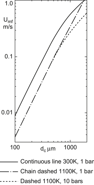
Figure 5.5 Superficial gas velocity of air at minimum fluidization, for spherical particles of density 2500 kg/m³ (Seville et al., 1997).

In Fig. 5.5, the continuous line represents values of U_mf at normal atmospheric conditions (300 K and 1 bar). Note the linearity of this log–log plot for small particle sizes, where U_mf is proportional to the square of diameter (Eq. (5.6)). Increase in temperature to 1100 K, shown by the dashed lines, increases the gas viscosity, which affects U_mf directly (see Eq. (5.6) again). Change in pressure has little effect for small particles but is important for larger ones, because it affects the gas density.

As regards fluidization behavior, the most important particle properties are density, size, and size distribution. The density of interest is what is sometimes called the “piece density” or “envelope density” (see Box 5.2). The average diameter to use is the surface-volume mean (see Chapter 3). This is the particle size whose surface area per unit mass or per unit solid volume is the average value for the whole particulate. It is therefore the best single measure of particle size for processes controlled by the interfacial area between gas and solids; this includes mass transfer processes and, to a first approximation, fluid/particle drag at low particle Reynolds numbers.

The relevant properties of the gas in a fluidized bed are its density ρ and viscosity μ. For virtually all practical purposes, the density of a gas or gas mixture can be estimated from the ideal gas laws; it is proportional to absolute pressure and inversely proportional to absolute temperature. To a good first approximation, the viscosity of a gas or gas mixture is independent of pressure but increases with increasing temperature; the variation is as T^½ according to elementary kinetic theory and is usually somewhat stronger in practice. Temperature can have an effect on the particles too, if it is high enough to cause sintering (time-dependent bonding) or melting.

Box 5.2 Which Density?

For a particulate solid, what is meant by “density”? The most basic meaning is the intrinsic density of the fully dense solid, which is a material property found in reference books. However, particles of that solid may have internal porosity, so the particle density may be much lower than the material density. The particles are then stored or transported in bulk, which introduces the idea of bulk density, which is lower still. For example, alumina has an intrinsic density of about 4000 kg/m³. As a porous catalyst carrier, this may be reduced to 2000 kg/m³ and the bulk density of the as-delivered material may be only 1000 kg/m³. Particle density is difficult to measure. This is normally done by a displacement method. More details are given in Chapter 2.

5.3.2. Bubbles

Most gas-fluidized beds operate in the bubbling regime. To a first approximation, in a bubbling fluidized bed only sufficient gas to support the particles flows in the small spaces (“interstices”) between the particles; this is termed the interstitial flow. Any excess passes through the bed as distinct bubbles. Taking the analogy with bubbles in liquids further, it is possible to distinguish between the dense phase (also known as the “particulate phase” or “emulsion phase”), consisting of the bed particles fluidized by the interstitial gas, and the lean phase, consisting of rising bubbles virtually free of bed particles.

A bubbling bed can be regarded as a bed in which the bubble phase is dispersed, and the particulate phase is continuous—as in a bubbling liquid. At higher gas velocity, the proportion of the bed volume occupied by the bubbles, ε_b, increases. It may become sufficiently high that the bed can no longer be described as “lean phase dispersed/particulate phase continuous.” The two “phases” are now so interspersed that neither can be described as continuous, sometimes known as “turbulent fluidization.” At higher velocities still, ε_b becomes so high that the “lean phase” is continuous, with the “particulate phase” dispersed in it.

Figure 5.6 shows an idealized section through a single bubble in a fluidized bed. The bubble volume is V_b. The upper surface is approximately spherical, with radius of curvature r. The base is typically indented. The volume filling in the sphere is called the wake and, to a good approximation, this volume V_W consists of dense phase rising with the bubble. Bubble shapes vary according to the properties of the bed particles, particularly their size; in general, the smaller the particles, the larger the ratio of wake volume to bubble volume.

The wake volume has an important effect on particle motion. The rising sphere, corresponding to the bubble plus its wake, displaces the surrounding dense phase; the effect is roughly equivalent to dragging up a volume equal to 1/2(V_b + V_W), by the process known as drift transport. If V_W = V_b/3, then the drift volume is roughly equal to 2V_b/3. Therefore, the total transport of dense phase, by drift and in the bubble wake, is

$2 V_{b} / 3 + V_{W} \approx 2 V_{b} / 3 + V_{b} / 3 = V_{b}$ $2 V_{b} / 3 + V_{W} \approx 2 V_{b} / 3 + V_{b} / 3 = V_{b}$

(5.8)

That is, to a first approximation, a bubble rising through a fluidized bed transports its own volume of dense phase. It is this rapid turnover of the bed particles which gives fluidized beds many of their important properties, such as good temperature uniformity.

The description above refers to isolated bubbles. Bubbles whose dimensions approach those of the bed behave rather differently and are known as slugs. Slugging is generally undesirable because slugs are not as effective at mixing the bed and they cause extreme pressure fluctuations, which may ultimately damage the equipment.

Theoretically, a large isolated bubble in a fluid of relatively low viscosity rises at velocity u_b (Davies and Taylor, 1950), where:

$u_{b} = 2 \sqrt{g r} / 3$ $u_{b} = 2 \sqrt{g r} / 3$

(5.9)

Bubble velocities in fluidized beds vary erratically, but Eq. (5.9) seems to give a good estimate for mean rise velocity. In a freely bubbling bed, the rise velocity is greater than the value given by Eq. (5.9), and this is discussed further below.

Usually the radius of curvature, r, is not known. The characteristic dimension frequently used is the volume-equivalent sphere diameter, d_v, i.e., the diameter of a sphere whose volume is equal to the bubble volume V_b. The rise velocity of an isolated bubble is then given by

$u_{b} = K \sqrt{g d_{v}}$ $u_{b} = K \sqrt{g d_{v}}$

(5.10)

where K depends on the relationship between r and d_v. Commonly, it is assumed that K = 0.71, as for bubbles in water, although values of 0.5–0.6 may be more realistic for smaller particles (below say 100 μm).

In a real bubbling fluidized bed, bubbles are seen to undergo both combination (“coalescence”) and splitting. Bubbles in fluidized beds break up by the process shown schematically in Fig. 5.7. An indentation forms on the upper surface of the bubble and grows as it is swept around the periphery by the particle motion. If the indentation grows sufficiently to reach the base of the bubble before being swept away, the bubble divides. Splitting dominates in beds of smaller particles (below say 100 μm) and also tends to become more frequent at higher pressures.

Figure 5.7 Bubble splitting. After Clift (1986).

Splitting leads to the idea of there being a maximum stable bubble size, which effectively limits the size to which they can grow. This size seems to be of order 1 cm for particles of size ∼60 μm, increasing to more than 1 m for particles of 250 μm, and over 10 m for particles of 1 mm in size. So in practice, splitting is only relevant for smaller particles.

When a bed of particles is fluidized at a gas velocity above the minimum bubbling point, bubbles form continuously and rise through the bed, which is said to be “freely bubbling.” Bubbles coalesce as they rise, so that the average bubble size increases with distance above the distributor (Fig. 5.3) until the bubbles approach the maximum stable size. For smaller particles, thereafter, splitting and recoalescence cause the average bubble size to equilibrate at a value close to the maximum stable value.

Bubble coalescence can also have an influence on circulation of the dense phase. The effect is shown schematically in Fig. 5.8. Bubbles usually coalesce by overtaking a bubble in front (Fig. 5.8(b)(i)) and may move sideways into the track of another bubble (Fig. 5.8(b)(ii)). Thus coalescence can cause lateral motion of bubbles. Bubbles near a bed wall can only move inward, because bubbles surrounding them are only on the side away from the wall, while bubbles well away from the walls are equally likely to move in any horizontal direction. As a result of this preferential migration of bubbles away from the wall, an “active” zone of enhanced bubble flow forms a small distance from the wall. In this zone, coalescence is more frequent so that the bubbles become larger than at other positions on the same horizontal plane. Because the region between the “active” zone and the wall is depleted of bubbles, coalescence continues to cause preferential migration toward the bed axis. Eventually the “active” zone comes together to form a “bubble track” along which the lean phase rises as a stream of large bubbles. Large beds may divide into several “cells,” with several preferential bubble tracks in the bed. Because of the transport of dense phase by the bubbles, the solids tend to move up in regions of high bubble activity and down elsewhere. In the upper levels, the motion is up near the bubble tracks and down near the walls. At lower levels, the particle motion is down near the axis and outward across the distributor; this motion can in turn enhance bubble activity near the walls close to the distributor.

Figure 5.8 (a) Bubbles and solids flow pattern and (b) coalescence behavior: (i) bubble overtaking; (ii) bubble sideways motion (Clift, 1986).

In design calculations it is necessary to predict bubble size and rise velocity, for which there are a number of empirical and semiempirical correlations. The approach due to Darton et al. (1977) has been shown to be reasonably reliable and is relatively convenient to use. The mean bubble size formed at the distributor d_v,o is first estimated by an expression whose form has a fundamental theoretical basis:

$d_{v,o} = 1.63 {(A_{o} (U - U_{mf}))}^{0.4} g^{- 0.2}$ $d_{v,o} = 1.63 {(A_{o} (U - U_{mf}))}^{0.4} g^{- 0.2}$

(5.11)

where A_o is the distributor area associated with one gas inlet orifice or nozzle. The effect of coalescence on bubble growth above the distributor is then given by

$d_{v} = 0.54 {(U - U_{mf})}^{0.4} {(z + 4 \sqrt{A_{o}})}^{0.8} g^{- 0.2}$ $d_{v} = 0.54 {(U - U_{mf})}^{0.4} {(z + 4 \sqrt{A_{o}})}^{0.8} g^{- 0.2}$

(5.12)

where z is the distance above the distributor. It is to be remembered, however, that for smaller particles the maximum bubble size is often reached quite close to the distributor, and this approach does not account for that effect.

The rise velocity of bubbles in a freely bubbling bed can be predicted approximately by the approach of Davidson and Harrison (1963), which gives the mean bubble rise velocity, u_A, as

$u_{A} = (U - U_{mf}) + u_{b}$ $u_{A} = (U - U_{mf}) + u_{b}$

(5.13)

where u_b is the rise velocity of a single isolated bubble (given by Eq. (5.10)). Instantaneous bubble velocities vary widely about this result and the mean velocity for a given bubble diameter varies with position in the bed, being highest in the “active” bubbling zones where coalescence is frequent.

5.3.3. Types of Fluidization

Early in the development of fluidization it was realized that the kind of fluidization behavior which can be achieved depends on the particle properties. For example, particles larger than about 1 mm tend to fluidize in a jerky, explosive sort of way while smaller particles fluidize much more smoothly. However, very small particles (say below 10 μm in size) do not fluidize at all, or only under special circumstances, apparently because their cohesive forces are so large compared with their particle weight (see Chapter 8).

There have been several attempts to devise theoretical and empirical classifications of fluidization behavior. Of these, the most widely used is the empirical classification of Geldart (1973), who divided fluidization behavior according to mean particle size and density difference between the solids and the fluidizing gas (Fig. 5.9). Geldart recognized four behavioral groups, designated A, B, C, and D. Typical fluidization behavior of groups A, B, and C is illustrated in Fig. 5.10.

Figure 5.9 Simplified diagram for classifying powders according to their fluidization behavior in air at ambient conditions (Geldart, 1973).

Group B (for “bubbling”) particles fluidize easily, with bubbles forming at or only slightly above the minimum fluidization velocity.

Group C (for “cohesive”) particles are cohesive and tend to lift as a plug or channel badly; conventional fluidization is usually difficult or impossible to achieve.

Group A particles are intermediate in particle size and in behavior between groups B and C and are distinguished from group B by the fact that appreciable (apparently homogeneous) bed expansion occurs above the minimum fluidization velocity but before bubbling is observed. There is now much experimental evidence that group A particles are also intermediate in cohesiveness between groups B and C, their interparticle cohesive forces being of the same order as the single particle weight.

Group D particles are those which are “large” and/or abnormally dense. Such particles fluidize poorly, but can be made to “spout,” rather than fluidize. A “spouted bed” is shown schematically in Fig. 5.11; its main features are a conical–cylindrical shape and a very pronounced solids circulation—up in the central lean “spout” and down in the dense annular ring around it. Gas is introduced through a small diameter entry at the base. This is not true fluidization because the gas does not support all the particles.

Typical properties associated with Geldart's groups are summarized in Table 5.2.

Figure 5.10 Typical fluidization behavior by Geldart groups B, A, and C (from left to right). Note that the scales are different for each group. After Seville (1987).

Figure 5.11 Solids circulation in a spouted bed (The length of the arrows is proportional to the average speed of the particles). Courtesy of Christian Seiler.

Table 5.2

Characteristic Features of Geldart's (1973) Classification of Fluidization Behavior (after Geldart, 1986)

Group	C	A	B	D
Typical examples	Flour, cement	Cracking catalyst	Building sand, table salt	Crushed limestone, coffee beans
Property
1. Bed expansion	Low when bed channels; can be high when fluidized	High	Moderate	Low
2. Deaeration rate	Can be very slow	Slow	Fast	Fast
3. Bubble properties	Channels	Splitting and coalescence predominate. Maximum size. Large wake.	No limit on size	No known upper size; small wake.
4. Solids mixing	Very low	High	Moderate	Low
5. Spouting	No, except in very shallow beds	Shallow beds only	Shallow beds only	Yes, even in deep beds

A different kind of classification of fluidization behavior due to Grace (1986) is shown in Fig. 5.12. This uses a dimensionless gas velocity, U^∗, and particle diameter,

d_{p}^{*}

$d_{p}^{*}$

as in Section 5.3.1, to define the behavioral groups, where

$d_{p}^{∗} = d_{p} {[\frac{ρ (ρ_{p} - ρ) g}{u^{2}}]}^{1 / 3}$ $d_{p}^{∗} = d_{p} {[\frac{ρ (ρ_{p} - ρ) g}{u^{2}}]}^{1 / 3}$

(5.14)

and

Figure 5.12 Regime/processing mode diagram, grouping systems according to type of powder and gas velocity used. After Grace (1986).

$U^{∗} = U {[\frac{ρ^{2}}{μ (ρ_{p} - ρ) g}]}^{1 / 3}$ $U^{∗} = U {[\frac{ρ^{2}}{μ (ρ_{p} - ρ) g}]}^{1 / 3}$

(5.15)

Figure 5.12 also shows the various processing options which might be considered for particles of various sizes and gases of different properties. Grace's classification successfully accounts for the effects of variation in gas properties due to operation at elevated temperature and pressure but there is, as yet, no satisfactory classification which also takes into account interparticle forces (see Chapter 8), which in many practical situations may be of considerable importance.

5.4. Pneumatic Conveying

As shown in Fig. 5.1, if the gas velocity is sufficient to carry the particles out of a fluidized bed, this is, in effect, a form of conveying, termed pneumatic conveying. In Fig. 5.1, vertical pneumatic conveying is shown. However, pneumatic conveying also operates horizontally, and at an angle to the vertical, although the last of these is not common.

In general, solid particles can be moved from place to place in bags, using forklift trucks and using mechanical devices such as screw conveyors and bucket elevators. Pneumatic conveying has advantages and disadvantages by comparison with these alternative methods. It requires low-operating labor input (runs unattended) and very little space. It also maintains the solids in a totally enclosed pipe so that contamination (both of the product and from the product) is prevented. Dispersed solids are an explosion risk (see, for example, Barton, 2002), but an inert gas can be used to convey the powder, which mitigates this risk. A disadvantage of pneumatic conveying is possible damage to the solids being conveyed, and/or erosion of the conveying pipe material, possibly causing contamination to the product.

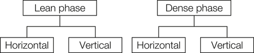
Pneumatic conveying systems fall into different categories, as shown in Table 5.3.

First, it is possible to convey solids in a fully dispersed state or as a more-or-less coherent dense plug. These approaches are termed “lean” and “dense” phase, respectively, where the dividing concentration is about 15 kg solid/kg gas. A further distinction lies in whether the conveying pipe is vertical or horizontal. Many systems contain both, of course, but the particle behavior is very different in the two directions, as discussed later. Finally, it is possible to blow powder along a pipe or up a column by exerting an excess pressure, or to suck a powder along a pipe under negative pressure (with respect to the atmosphere), as in a domestic vacuum cleaner. It is also possible to have systems which employ a combination of “blow” and “suck.” Examples of such systems are given below.

Table 5.3

Categorizing Pneumatic Conveying Systems

The design process for pneumatic conveying can be summarized as:

• Choose a conveying system type

• Choose a gas velocity which is high enough to transport the solids but low enough not to be too costly (or too damaging to the solids)

One guide to selection of pneumatic conveying systems (from the company Neu Engineering) recommends the following:

1. System duty

a. Choose low pressure systems for conveying duties up to 10 t/h and up to 150 m in distance.

b. Choose high pressure systems for conveying duties up to 50 t/h and up to 500 m in distance.

2. Process layout

a. If there are multiple sources of solids to be considered, choose a suction system

b. If there are multiple destinations for solids to be considered, choose a blowing system

c. If there are multiple sources and destinations to be considered, choose a combination suck–blow system

In addition to these selection criteria there are obviously also product considerations, some of which are summarized in Table 5.4.

Figures 5.13–5.15 show three examples of pneumatic conveying systems.

Figure 5.13 shows a typical pressurized system in which blowers are used to pressurize a transport tanker and convey particles—in this case flour—from the tanker to two storage silos, from which they can be further transported to a sieving unit.

Table 5.4

Product Considerations in Pneumatic Conveying

Product	System choice
Toxic	Suction usually
Explosive	Inert gas/positive pressure
Large particle size	Low pressure
Fragile	Low velocity/dense phase
Abrasive	Low velocity/dense phase
Cohesive/damp	Slug phase
Temperature-sensitive	Suction
Hygroscopic	Positive pressure

Figure 5.13 Blow-type flour delivery system, with aerated silos. Courtesy of Neu Engineering.

Figure 5.14 Solid fuel/ash handling system. Courtesy of Neu Engineering.

Figure 5.15 Multiple source/multiple destination food mix system. Courtesy of Neu Engineering.

Figure 5.14 shows a typical suction system in which a pelletized solid fuel is sucked up from a storage pit into two cyclones situated above combustion chambers, where the solids are separated into the gas and fed into the chambers. In a separate system, ash falls under gravity from underneath the combustion chambers, where it is conveyed under pressure to a filter situated above a storage silo, from which the ash can be taken away by truck.

Figure 5.15 shows a very flexible system in which solids can be extracted under suction from a combination of ingredient silos, shown on the left, into a filter situated above a metering silo from which the particles are conveyed under pressure to a mixing vessel (also shown being fed with a small mass ingredient using a separate screw conveyor).

It will be apparent from the designs shown here that there are a number of auxiliary devices needed to make up a pneumatic conveying system, including devices to introduce the solids to the gas, such as eductors, rotary valves, and blow tanks (see Fig. 5.16), and devices to separate the solids from the gas, such as cyclones and filters (considered in Section 5.5).

The pressure drop versus gas velocity relationships for pneumatic conveying are complex. In general, the pressure drop in a system has six constituent terms, which are due to:

• Acceleration of the gas (proportional to ρU²)—usually small

• Acceleration of the particles (proportional to

ρ_{s} U_{s}^{2}

$ρ_{s} U_{s}^{2}$

)—could be large

• Gas-to-pipe friction—usually small

• Solids-to-pipe friction—usually large

• Static head of gas (ρHg)—usually small

• Static head of solids (ρ_sU(1−ε)Hg)—large if vertical

where ρ and ρ_s are the gas and particle densities, U and U_s are the gas and particle velocities, ε is the void fraction, H is the vertical conveying height, and g is the acceleration due to gravity.

Figure 5.16 Devices for introducing particulate solids to a gas stream.

From this comparison it is possible to say that the largest contributions to pressure drop are likely to be due to the solids—their initial acceleration as they are introduced to the flowing gas by a rotary valve or alternative device, their pipe friction due to repeated collisions with the wall and their consequent loss of momentum, and their static head contribution in vertical conveying. Figure 5.17 shows the first two of these effects schematically.

Figure 5.17 Pressure drop in horizontal conveying—acceleration loss and friction loss. After Seville et al. (1997).

Figure 5.18 shows the pressure drop versus gas velocity behavior to be expected in vertical conveying. The curves represent constant values of the solids mass flow rate, with the lowest one representing gas flow only. Consider what happens as the gas velocity is reduced with the solids flow rate kept constant: the in situ particle concentration goes up so that the “hydrostatic” contribution to the pressure gradient goes up. This contribution eventually outweighs the decrease in the frictional pressure gradient, so that the total gradient passes through a minimum and then increases. Eventually it rises more sharply, to a condition in which the riser pipe contains a slugging (or, more rarely, bubbling) fluidized bed. This condition is called choking. A “choked” vertical conveying line is typically characterized by pressure fluctuations, associated with the rise and eruption of slugs. As for horizontal conveying, the transition velocity depends on the solids flow rate.

Figure 5.19 shows the different modes which can be observed in horizontal conveying, while Fig. 5.20 shows the pressure drop versus gas velocity behavior. In horizontal flow, the transition from lean- to dense-phase flow is usually termed the saltation velocity. At constant solids flow rate, G, and starting with a high superficial high gas velocity, U, the mixture is in lean-phase flow. If the gas flow is reduced, the pressure gradient at first decreases as the frictional contribution is reduced. When the saltation velocity (U_salt) is reached, the pressure gradient increases sharply, which indicates a transition to dense-phase flow. Further reduction in gas flow causes the pressure gradient to increase further. The reverse transition occurs on increasing flow, without appreciable hysteresis if the flow is allowed to reach steady state. The saltation velocity increases when the solids flow rate is increased. Therefore, the transition from lean to dense flow may be triggered by an increase in solids flow rate, if the line is operating close to the saltation point.

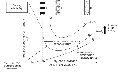
Figure 5.18 Phase diagram for vertical conveying. After Knowlton (1986).

Figure 5.19 Horizontal pneumatic conveying regimes.

Figure 5.20 Phase diagram for horizontal pneumatic conveying. After Knowlton (1986).

Pneumatic systems often contain bends, which can have a substantial effect on the pressure drop because the solids can be knocked out of the flow and have to be resuspended. Figure 5.21 shows a schematic illustration of this.

Figure 5.21 Schematic of pressure drop at a bend in pneumatic conveying.

5.5. Gas–Solid Separation^∗

The separation of particles from gases is an important technical problem in engineering and has applications in many industries, both for environmental protection and for prevention of fouling and damage to equipment. The devices which have been proposed to achieve this separation are astonishingly varied in design, in the physical principles upon which they rely, and in their effectiveness. For example, such devices include

• Cyclones, in which the particles are separated by aerodynamic effects

• Filters, in which particles are mechanically separated from the gas, which is forced to pass through some sort of porous material

• Wet scrubbers, in which the particles are separated by being captured in droplets or films of liquid

• Electrostatic precipitators, in which the particles are charged and then caused to migrate in an electric field to collection plates

This chapter concerns only the first two of these devices—the cyclone and the filter—which are by far the most commonly used.

5.5.1. Cyclones

The cyclone is an example of a generic device termed an inertial separator. Inertial separators concentrate or collect particles by changing the direction of motion of the flowing gas, in such a way that the particle trajectories cross over the gas steamlines so that the particles are either concentrated into a small part of the gas flow or are separated by making contact with a surface. In a cyclone the gas undergoes some kind of vortex motion so that the gas acceleration is centripetal, and the particles therefore move centrifugally towards the outside of the cyclone.

Figure 5.22 shows the most important features of a typical reverse-flow cyclone, where the vortex motion is induced by introducing the gas tangentially to a cylindrical section called the cyclone barrel. The gas exits through an axial pipe sometimes called the vortex finder. The end of the vortex finder extends beyond the gas outlet, so that the gas executes a helical outer vortex in the barrel and tapered section or cone, before moving into the much narrow inner vortex and leaving through the vortex finder. The particles are flung out to the wall while, in a properly designed cyclone, the helical motion in the outer vortex pushes them down toward the apex of the cone. Most commonly, cyclones are mounted vertically for easier discharge of particles from the cone, but they can be (and sometimes are) used in different orientations. A disengagement hopper is sometimes provided to control particle discharge, as shown in Fig. 5.22. However, in some applications where the particles are retained within the process, a dip-leg is used instead, in the form of a pipe down which the disengaged particles move in dense-phase flow. This is common practice in collecting particles from the gases leaving fluidized bed reactors or combustors, for example, and the dip-leg then usually extends down below the surface of the bed.

Figure 5.22 A typical reverse-flow cyclone, showing gas motion. After Strauss (1975).

The gas entry to the cyclone is critical. It is preferable to ensure a sufficient length of straight pipe—at least several pipe diameters—before entering the cyclone. The different gas entry configurations are exemplified by the archetypal designs of Stairmand³ (e.g., 1951, 1955) shown in Fig. 5.23, which are almost “industry standards.” A simple tangential entry, shown in Fig. 5.23(a), is cheaper to construct but may give higher pressure drop across the cyclone (see below); Stairmand used the tangential entry for his “high efficiency, medium throughput” design. For lower pressure drop (but increased construction cost), a volute (or “scroll” or “wrap-around”) entry can be used, as in Stairmand's “high throughput, medium efficiency” design shown in Fig. 5.23(b).

Figure 5.23 Standard cyclone designs. Strauss (1975); after Stairmand (1951).

Other types of inertial separator have been suggested and some, such as axial-entry types with swirl vanes for air-intakes, have become popular in some specialized applications, but types based on the two basic designs shown in Fig. 5.23 remain commonly used.

It is possible to analyze particle motion in cyclones using various mechanistic and computational approaches, but for design work it is much easier to resort to the common practice of dimensional analysis. For most purposes, this is quite adequate, because reputable cyclone suppliers have good data on performance which can readily be scaled or extrapolated using appropriate dimensionless groups.

5.5.1.1. Dimensional Analysis of Cyclone Performance

When particles are separated from a gas this is termed collection. The efficiency of particle collection, η, by an inertial separator, operated at given gas properties and throughput, depends on particle diameter, d, and density, ρ_p. The relationship between η and d for given ρ_p is called the grade efficiency curve. Grade efficiency curves for the two Stairmand designs of Fig. 5.23 are shown in Fig. 5.24. These curves refer to low inlet particle loading in the inlet gas (mass of solids per mass of gas); the effect of increasing particle loading is to increase efficiency, so designs using this approach should be conservative. A simple scaling approach can now be used to apply measured grade efficiency curves to different conditions and different sizes of cyclones.

Figure 5.24 Grade efficiencies for standard cyclones. Strauss (1975); after Stairmand (1951).

The collection efficiency for a particle of diameter d depends on the following variables:

$η = f [d, ρ_{p}, ρ, μ, D, Q]$ $η = f [d, ρ_{p}, ρ, μ, D, Q]$

(5.16)

where D is the characteristic cyclone dimension, typically the barrel diameter, and Q is the gas volumetric flow rate. Proceeding as above, the problem can be generalized by writing it in terms of six minus three, i.e., three dimensionless groups. (Collection efficiency is already dimensionless.) Hence we can write:

$η = f [St, Re, d / D]$ $η = f [St, Re, d / D]$

(5.17)

where St is the Stokes number derived from the ratio of the stopping distance (see Chapter 4) to cyclone diameter:

$St = \frac{ρ_{p} d^{2} U_{e}}{18 μ D} = \frac{2}{9 π} \frac{ρ_{p} d^{2} Q}{μ D^{3}}$ $St = \frac{ρ_{p} d^{2} U_{e}}{18 μ D} = \frac{2}{9 π} \frac{ρ_{p} d^{2} Q}{μ D^{3}}$

(5.18)

However, Eq. (5.17) can be simplified. In practice, cyclones operate at very high Reynolds number so that, as for many devices which operate in the fully turbulent flow range, the effect of changes in Reynolds number can be neglected. Similarly the size ratio, d/D, is usually so small that its effect can be ignored. This leaves:

$η = f [St]$ $η = f [St]$

(5.19)

Equation (5.19) shows that the grade efficiency can be put into a general nondimensional form by expressing η as a function of St rather than d. In particular, the particle size which can be collected by a cyclone is commonly expressed in terms of the cut size, d₅₀, i.e., the particle size which is collected (at low particle loading) with 50% efficiency, η = 0.5. From Eqs (5.18) and (5.19), for a given geometric cyclone design,

$\frac{ρ_{p} d_{50}^{2} Q}{μ D^{3}} = constant$ $\frac{ρ_{p} d_{50}^{2} Q}{μ D^{3}} = constant$

(5.20)

$d_{50} \propto \sqrt{(μ D^{3} / ρ_{p} Q)}$ $d_{50} \propto \sqrt{(μ D^{3} / ρ_{p} Q)}$

(5.21)

Equation (5.21) shows that the cut size decreases (i.e., the cyclone efficiency improves) if the throughput increases, and also that the performance of small cyclones is better than that of large cyclones, all other things being equal (Box 5.3).

A similar dimensional approach can be taken to prediction of the pressure drop across the cyclone, ΔP, which depends on the cyclone dimensions, the gas volumetric flow rate, Q, and the gas density and viscosity, ρ and μ:

$Δ P = f [D, Q, ρ, μ]$ $Δ P = f [D, Q, ρ, μ]$

(5.22)

Equation (5.22) applies for the gas flow alone; particle loading effects are discussed below. Given the five parameters in Eq. (22) and that the system has the usual three dimensions (mass, length, and time), the problem can be expressed in terms of two (i.e., five minus three) dimensionless groups. These are, most conveniently, the pressure coefficient:

Box 5.3 Cyclone Scaling

Equation (5.20) is extremely useful for design purposes, since it means that the performance of any size of cyclone under any conditions of gas flow can be predicted from that of a geometrically similar cyclone for which experimental data are available. So, for the two cyclones shown below,

$S t_{50} = {[d_{50}^{2} ρ_{p} U / 18 μ D]}_{A} = {[d_{50}^{2} ρ_{p} U / 18 μ D]}_{B}$ $S t_{50} = {[d_{50}^{2} ρ_{p} U / 18 μ D]}_{A} = {[d_{50}^{2} ρ_{p} U / 18 μ D]}_{B}$

$Π = Δ Ρ / (ρ U_{e}^{2} / 2) = \frac{π^{2} D^{4} Δ P}{8 Q^{2} ρ}$ $Π = Δ Ρ / (ρ U_{e}^{2} / 2) = \frac{π^{2} D^{4} Δ P}{8 Q^{2} ρ}$

(5.23)

and a cyclone Reynolds number:

${Re}_{c} = \frac{ρ U_{e} D}{μ} = \frac{4 ρ Q}{π μ D}$ ${Re}_{c} = \frac{ρ U_{e} D}{μ} = \frac{4 ρ Q}{π μ D}$

(5.24)

so that, for a given cyclone geometry,

$Π = f [{Re}_{c}]$ $Π = f [{Re}_{c}]$

(5.25)

In these equations, U_e represents a superficial velocity through the cyclone:

$U_{e} = Q / (π D^{2} / 4)$ $U_{e} = Q / (π D^{2} / 4)$

(5.26)

and is used here as a measure of gas velocity. The inlet velocity is typically of order 10U_e, the precise value depending on the geometric design of the cyclone.

The effective value of Π depends on the cyclone design; for geometrically similar cyclones over the normal velocity range, Π is approximately constant.

In practice, cyclones are often operated in combination, both in parallel (with the flow split between several cyclones) and in series (so that the larger particles are collected by the first cyclone, with progressively smaller particles collected by subsequent cyclones designed to have a smaller cut size). A discussion on multi-cyclone systems is presented in Box 5.4.

5.5.2. Filters

Filtration is the commonest method of particle removal from a fluid and refers to the process by which the particle-laden gas passes through a permeable membrane or an array of fibers, commonly termed the filter “medium.”

Commonly-used filter media include woven and nonwoven fabrics, paper, ceramics, metals in various forms, and granular materials. An example of a nonwoven filter material is shown in Fig. 5.25. In industrial use, filters often consist of arrays of vertically hung cylindrical elements (“bags” in the case of flexible fabric filters; “candles” in the case of rigid media) as shown in Fig. 5.26. The flow is from the outside inward and exits via a plenum chamber at the top. Many other geometries are known.

A distinction can be drawn between two main types of filtration behavior: depth filtration and surface or barrier filtration (Fig. 5.27). In depth filtration, collection of particles from the gas occurs throughout the filter medium. The two main mechanisms by which this happens (Fig. 5.28) are diffusional collection and inertial collection. In diffusional collection, particles deviate from the gas streamlines in a “random walk,” due to molecular impacts; in inertial collection, particles deviate from the streamlines because of their inertia. Diffusion decreases as the particle size increases, while inertia increases with size. The combination of the two effects is shown in Fig. 5.29. Large and small particles are collected with high efficiency, but there is a minimum efficiency at the “most penetrating size,” typically about 1 μm.

Box 5.4 MULTI-Cyclone Systems

For given gas and particle properties (i.e., ρ, μ, and ρ_p fixed) from Eq. (5.23)

$Δ P \propto Q^{2} / D^{4}$ $Δ P \propto Q^{2} / D^{4}$

(5.27)

while, from Eq. (5.21),

$d_{50} \propto {(D^{3} / Q)}^{1 / 2} \propto D^{1 / 2} Δ P^{- 1 / 4}$ $d_{50} \propto {(D^{3} / Q)}^{1 / 2} \propto D^{1 / 2} Δ P^{- 1 / 4}$

(5.28)

so that lower d₅₀ (i.e., improved collection performance) can also be achieved at the expense of higher pressure drop.

The analysis above also explains the use of a number of identical cyclones in parallel. For N cyclones handling a total gas flow rate Q, the flow per cyclone should be

$q = Q / N$ $q = Q / N$

(5.29)

so that, from Eq. (5.21)

$Δ P \propto q^{2} / D^{4} \propto Q^{2} / N^{2} D^{4}$ $Δ P \propto q^{2} / D^{4} \propto Q^{2} / N^{2} D^{4}$

(5.30)

To maintain collection performance, from Eq. (5.27) D³/q must be kept constant; i.e., ND³/Q must be constant, implying that

$D^{3} \propto N^{- 1}$ $D^{3} \propto N^{- 1}$

(5.31)

for given total flow rate Q. From Eqs (5.30) and (5.31)

$Δ P \propto Q^{2} N^{- 2 / 3}$ $Δ P \propto Q^{2} N^{- 2 / 3}$

(5.32)

That is, for given collection performance, the pressure drop can be reduced by using a number of cyclones in parallel. In practice, the number of parallel cyclones is limited by the difficulty of ensuring uniform gas distribution between them, although this general result explains the interest in devices using batteries of small cyclones in parallel, usually of an axial flow design.

Figure 5.25 Scanning electron microscope picture of a nonwoven polyester filter cloth. Courtesy of Freudenberg.

Figure 5.26 A typical bag filter arrangement (Barton, 2002).

Figure 5.27 Surface and depth filtration—schematic.

Figure 5.28 Diffusional collection (left) and inertial collection (right). The larger sphere represents an element of the filter medium.

Figure 5.29 Typical grade efficiency for depth filtration in a fibrous medium (both scales are logarithmic).

In surface filtration, the medium acts as a barrier to the solids so that a dust “cake” is built up on the upstream surface (Fig. 5.30), with no penetration into the medium itself. In practice, filtration behavior depends on the properties of both the dust and the medium, not only the relative size of the pores in the medium but also the surface properties (such as adhesion) of both. In general, gas cleaning using membranes and the finer grades of fibrous and granular filtration media approximates to surface filtration. Perfect surface filtration is rare, and with a new “surface filter” it is usual for there to be a short period of penetration into the surface layers of the medium before cake formation begins. During this short period the filtration efficiency may be lower than in steady operation.

Figure 5.30 Dust cake build up on a fibrous filter. (A section through a polyester needle felt filter of fiber diameter about 13 μm, with a limestone dust; courtesy of Eberhard Schmidt, Institute of Particle Technology, University of Wuppertal.)

In depth filtration it is not usually possible to remove particles effectively from the filter after they have been captured, certainly not “on line” (i.e., without shutting down the filter and removing the filtration medium). Barrier filters, however, are usually cleaned in situ, sometimes by shaking or other mechanical action but more commonly by gas flow in the opposite direction to that of the filtration flow.

In general, barrier filters are operated cyclically (Fig. 5.31). During filtration, dust builds up on the filter. After a prescribed time, or when the resistance to flow reaches a prescribed level, the medium is cleaned. The usual cleaning action is a reverse pulse of gas, applied to the clean side of the filter while it is on line. This detaches the cake of deposited particles, which then falls into a collecting hopper at the base of the unit, and the cycle is restarted. During the first few cycles, the “residual pressure drop” (after cleaning) increases, but after some time in a well-designed filter it usually levels off, as shown.

The most important design relationship for filters is that between pressure drop and gas velocity. In a filter the usual velocity which is chosen is the face velocity or the total volumetric flow at filtration conditions divided by the surface area of the filter which is available for flow. For a cylindrical bag, for example, this surface is the sum of the outer surface of the cylinder plus the end cap.

The total pressure drop of a surface filter is due to the resistance of the filter medium plus the resistance of the dust cake; the latter may be much larger than the former. To complicate matters further, even after pulse cleaning, the resistance of the medium does not return to its original value, as shown in Fig. 5.31. This effect is very system-specific.

Figure 5.31 Cyclic behavior of a pulse-cleaned barrier filter.

Nevertheless, it is of interest to determine the pressure drop of the clean filter medium for comparison purposes. In general, the pressure drop through a planar porous medium can be represented (see Eq. (5.1)) as

$- \frac{ⅆ P}{ⅆ z} = k_{1} μ U + k_{2} ρ U^{2}$ $- \frac{ⅆ P}{ⅆ z} = k_{1} μ U + k_{2} ρ U^{2}$

(5.33)

where (−dP/dz) is the pressure gradient in the direction of flow, and U is the superficial fluid velocity, i.e., the actual volumetric flow rate divided by the area available for flow. In the case of the media considered here, the Reynolds number (Uρd_p/μ) is much less than unity, so that the second term in Eq. (5.33) can be neglected, and k₁ can be replaced by the Kozeny expression provided that the void fraction ε is not too high (Kyan et al., 1970):

$k_{1} = k_{k} {(1 - ε)}^{2} ε^{- 3} S_{o}^{2}$ $k_{1} = k_{k} {(1 - ε)}^{2} ε^{- 3} S_{o}^{2}$

(5.34)

where ε is the void fraction, S_o the specific surface area of the medium, and K_k is the Kozeny parameter, which depends on the geometrical structure. Equation (5.34) can be used to “design” a medium with the desired resistance characteristics. In cases where ε > 0.95, such as in many fibrous media, the prediction of pressure drop is much more complex; reviews are presented by Strauss (1975) and Brown (1993).

..................Content has been hidden....................

You can't read the all page of ebook, please click here login for view all page.

Table of Contents for Chapter 5. Gas–Solid Systems

Create new playlist

Sign In

Sign Up