
Sooner or later, we’ll all face a query that takes just a bit longer to execute than what we have patience for. The best and easiest fix to a sluggish query is to perfect the underlying SQL, followed by adding indexes, and updating planner statistics. To guide you in these pursuits, Postgres comes with a built-in explainer that informs you how the query planner is going to execute your SQL. Armed with your knack for writing flawless SQL, your instinct to sniff out useful indexes, and the insight of the explainer, you should have no trouble getting your queries to run as fast as what your hardware budget will allow.
The easiest tool for targeting query performance problems is using
the EXPLAIN and EXPLAIN ANALYZE commands. These
have been around ever since the early years of PostgreSQL. Since then it
has matured into a full-blown tool capable of reporting highly detailed
information about the query execution. Along the way, it added to its
number of output formats. In PostgreSQL 9.0+, you can even dump the output
to XML or JSON. Perhaps the most exciting enhancement for the common user
came when pgAdmin introduced graphical EXPLAIN several years
back. With a hard and long stare, you can identify where the bottlenecks
are in your query, which tables are missing indexes, and whether the path
of execution took an unexpected turn.
EXPLAIN will give you just an idea of how the planner
intends to execute the query without running it. EXPLAIN
ANALYZE will actually execute the query and give you comparative
analysis of expected versus actual. For the non-graphical version of
EXPLAIN, simply preface your SQL with the
EXPLAIN or EXPLAIN ANALYZE. VERBOSE
is an optional modifier that will give you details down to the columnar
level. You launch graphical EXPLAIN via pgAdmin. Compose the
query as usual, but instead of executing it, choose EXPLAIN
or EXPLAIN ANALYZE from the drop down menu.
Note
It goes without saying that to use graphical explain, you’ll need more than a command prompt. To those of you who pride yourself on being self-sufficient using only the command line: good for you!
Let’s try an example, we’ll first use the EXPLAIN
ANALYZE command.
Example 9-1. Explain analyze
EXPLAIN ANALYZE SELECT left(tract_id,5) As county_code, SUM(hispanic_or_latino) As tot , SUM(white_alone) As tot_white , SUM(coalesce(hispanic_or_latino,0) - coalesce(white_alone,0)) AS non_white FROM census.hisp_pop GROUP BY county_code ORDER BY county_code;
The output of Example 9-1 is shown in Example 9-2.
Example 9-2. EXPLAIN ANALYZE output
GroupAggregate (cost=111.29..151.93 rows=1478 width=20)
(actual time=6.099..10.194 rows=14 loops=1)
-> Sort (cost=111.29..114.98 rows=1478 width=20)
(actual time=5.897..6.565 rows=1478 loops=1)
Sort Key: ("left"((tract_id)::text, 5))
Sort Method: quicksort Memory: 136kB
-> Seq Scan on hisp_pop (cost=0.00..33.48 rows=1478 width=20)
(actual time=0.390..2.693 rows=1478 loops=1)
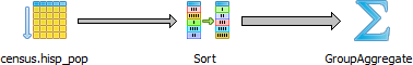
Total runtime: 10.370 msIf reading the output is giving you a headache, here’s the graphical
EXPLAIN:
Before leaving the section on EXPLAIN, we must pay
homage to a new online
EXPLAIN tool created by Hubert “depesz” Lubaczewski.
Using his site, you can copy and paste the text output of your
EXPLAIN, and it will show you a beautifully formatted stats
report as shown in Figure 9-2.
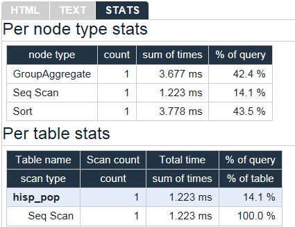
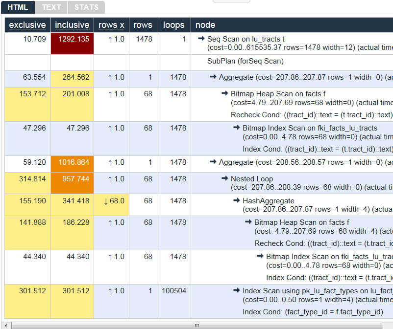
In the HTML tab, a nicely reformatted color-coded table of the plan will be displayed, with problem areas highlighted in vibrant colors, as shown in Figure 9-3.
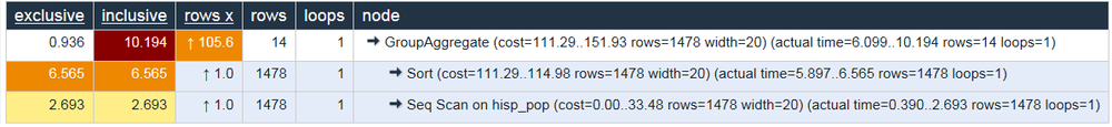
Although the HTML table in Figure 9-3 provides much the same information as our plain-text plan, the color coding and breakout of numbers makes it easier to see that our actual values are far off from the estimated numbers. This suggests that our planner stats are probably not up to date.
The best and easiest way to improve query performance is to start with well-written queries. Four out of five queries we encounter are not written as efficiently as they could be. There appears to be two primary causes for all this bad querying. First, we see people reuse SQL patterns without thinking. For example, if they successfully write a query using a left join, they will continue to use left join when incorporating more tables instead of considering the sometimes more appropriate inner join. Unlike other programming languages, the SQL language does not lend itself well to blind reuse. Second, people don’t tend to keep up with the latest developments in their dialect of SQL. If a PostgreSQL user is still writing SQL as if he still had an early version, he’d be oblivious to all the syntax-saving (and mind-saving) addendums that have come along. Writing efficient SQL takes practice. There’s no such thing as a wrong query as long as you get the expected result, but there is such a thing as a slow query. In this section, we’ll go over some of the common mistakes we see people make. Although this book is about PostgreSQL, our constructive recommendations are applicable to other relational databases as well.
A classic newbie mistake is to think about a query in independent pieces and then trying to gather them up all in one final SELECT. Unlike conventional programming, SQL doesn’t take kindly to the idea of blackboxing where you can write a bunch of subqueries independently and then assemble them together mindlessly to get the final result. You have to give your query the holistic treatment. How you piece together data from different views and tables is every bit as important as how you go about retrieving the data in the first place.
Example 9-3. Overusing subqueries
SELECT tract_id
,(SELECT COUNT(*) FROM census.facts As F
WHERE F.tract_id = T.tract_id) As num_facts
,(SELECT COUNT(*) FROM census.lu_fact_types As Y
WHERE Y.fact_type_id IN (SELECT fact_type_id
FROM census.facts F WHERE F.tract_id = T.tract_id)) As num_fact_types
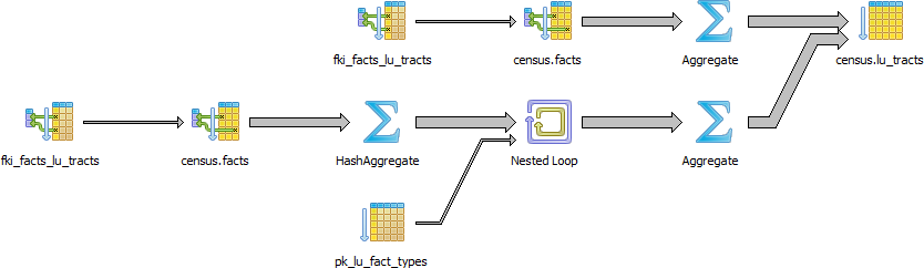
FROM census.lu_tracts As T;The graphical EXPLAIN plan for Example 9-3 is shown in Figure 9-4.
We’ll save you the eyesore from seeing the gnarled output of the
non-graphical EXPLAIN. Instead, we’ll show you in Figure 9-5 the output from using the
online EXPLAIN at http://explain.depesz.com.
Example 9-3 can be more efficiently written as shown in Example 9-4. This version of the query is not only shorter, but faster than the prior one. If you have even more rows or weaker hardware, the difference would be even more pronounced.
Example 9-4. Overused subqueries simplified
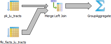
SELECT T.tract_id, COUNT(f.fact_type_id) As num_facts, COUNT(DISTINCT fact_type_id) As num_fact_types FROM census.lu_tracts As T LEFT JOIN census.facts As F ON T.tract_id = F.tract_id GROUP BY T.tract_id;
The graphical EXPLAIN plan of Example 9-4 is shown in Figure 9-6.
Keep in mind that we’re not asking you to avoid subqueries. We’re simply asking you to use them judiciously. When you do use them, be sure to pay extra attention on how you combine them into the main query. Finally, remember that a subquery should try to work with the the main query, not independent of it.
SELECT * is wasteful. It’s akin to printing out a
1,000-page document when you only need ten pages. Besides the obvious
downside of adding to network traffic, there are two other drawbacks
that you might not think of.
First, PostgreSQL stores large blob and text objects using TOAST
(The Oversized-Attribute Storage Technique). TOAST maintains side tables
for PostgreSQL to store this extra data. The larger the data the more
internally divided up it is. So retrieving a large field means that
TOAST must assemble the data across different rows across different
tables. Imagine the extra processing should your table contain text data
the size of War and Peace and you
perform an unnecessary SELECT *.
Second, when you define views, you often will include more columns
than you’ll need. You might even go so far as to use SELECT
* inside a view. This is understandable and perfectly fine.
PostgreSQL is smart enough that you can have all the columns you want in
your view definition and even include complex calculations or joins
without incurring penalty as long as you don’t ask for them.
SELECT * asks for everything. You could easily end up
pulling every column out of all joined tables inside the view.
To drive home our point, let’s wrap our census in a view and use the slow subselect example we proposed:
CREATE OR REPLACE VIEW vw_stats AS
SELECT tract_id
,(SELECT COUNT(*) FROM census.facts As F WHERE F.tract_id = T.tract_id) As num_facts
,(SELECT COUNT(*) FROM census.lu_fact_types As Y
WHERE Y.fact_type_id
IN (SELECT fact_type_id FROM census.facts F
WHERE F.tract_id = T.tract_id)) As num_fact_types
FROM census.lu_tracts As T;Now if we query our view with this query:
SELECT tract_id FROM vw_stats;
Execution time is about 21ms on our server. If you looked at the plan, you may be startled to find that it never even touches the facts table because it’s smart enough to know it doesn’t need to. If we used the following:
SELECT * FROM vw_stats;
Our execution time skyrockets to 681ms, and the plan is just as we had in Figure 9-4. Though we’re looking at milliseconds still, imagine tables with tens of millions of rows and hundreds of columns. Those milliseconds could transcribe into overtime at the office waiting for a query to finish.
We’re always surprised how frequently people forget about using
the ANSI-SQL CASE expression. In many aggregate situations,
a CASE can obviate the need for inefficient subqueries.
We’ll demonstrate with two equivalent queries and their corresponding
plans.
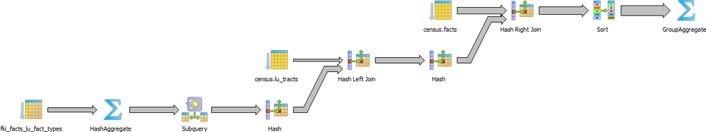
Example 9-5. Using subqueries instead of CASE
SELECT T.tract_id, COUNT(*) As tot, type_1.tot AS type_1
FROM census.lu_tracts AS T
LEFT JOIN
(SELECT tract_id, COUNT(*) As tot
FROM census.facts WHERE fact_type_id = 131
GROUP BY tract_id) As type_1 ON T.tract_id = type_1.tract_id
LEFT JOIN census.facts AS F ON T.tract_id = F.tract_id
GROUP BY T.tract_id, type_1.tot;The graphical explain of Example 9-5 is shown in Figure 9-7.
We now rewrite the query using CASE. You’ll find the
revised query shown in Example 9-6 is generally faster and
much easier to read than Example 9-5.
Example 9-6. Using CASE instead of subqueries
SELECT T.tract_id, COUNT(*) As tot , COUNT(CASE WHEN f.fact_type_id = 131 THEN 1 ELSE NULL END) AS type_1 FROM census.lu_tracts AS T LEFT JOIN census.facts AS F ON T.tract_id = F.tract_id GROUP BY T.tract_id;
The graphical explain of Example 9-6 is shown in Figure 9-8.
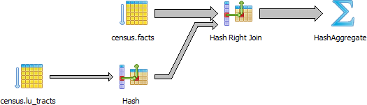
Even though our rewritten query still doesn’t use the fact_type index, it’s still generally faster than using subqueries because the planner scans the facts table only once. Although not always the case, a shorter plan is generally not only easier to comprehend, but also performs better than a longer one.
The planner’s behavior is driven by several cost settings, strategy settings, and its general perception of the distribution of data. Based on distribution of data, the costs it ascribes to scanning indexes, and the indexes you have in place, it may choose to use one strategy over another. In this section we’ll go over various approaches for optimizing the planner’s behavior.
Although PostgreSQL query planner doesn’t provide the option to accept index hints like some other databases, when running a query you can disable various strategy settings on a per query or pemanent basis to dissuade the planner from going down an unproductive path. All planner optimizing settings are documented in the section Planner Method Configuration. By default, all strategy settings are enabled, giving the planner flexibility to maximize the choice of plans. You can disable various strategies if you have some prior knowledge of the data. Keep in mind that disabling doesn’t necessarily mean that the planner will be barred from using the strategy. You’re only making a polite request to the planner to avoid it.
Two of our favorite method settings to disable are the
enable_nestloop and
enable_seqscan. The reason is that these two
strategies tend to be the slowest and should be relegated to be used
only as a last resort. Although you can disable them, the planner may
still use them when it has no other viable alternative. When you do see
them being used, it’s a good idea to double-check that the planner is
using them out of necessity, not out of ignorance. One quick way to
check is to actually disable them.
When the planner decides to perform a sequential scan, it plans to loop through all the rows of a table. It will opt for this route if it finds no index that could satisfy a query condition, or it concludes that using an index is more costly than scanning the table. If you disable the sequential scan strategy, and the planner still insists on using it, then it means that the planner thinks whatever indexes you have in place won’t be helpful for the particular query or you are missing indexes altogether. A common mistake people make is they write queries and either don’t put indexes in their tables or put in indexes that can’t be used by their queries. An easy way to check if your indexes are used is to query the pg_stat_user_indexes and pg_stat_user_tables views.
Let’s start off with a query against the table we created in Example 6-7. We’ll add a
GIN index on the array column. GIN
indexes are one of the few indexes you can use with arrays.
CREATE INDEX idx_lu_fact_types ON census.lu_fact_types USING gin (fact_subcats);
To test our index, we’ll execute a query to find all rows with
subcats containing “White alone” or “Asian alone”. We explicitly enabled
sequential scan even though it’s the default setting, just to be sure.
The accompanying EXPLAIN output is shown in Example 9-7.
Example 9-7. Allow choice of Query index utilization
set enable_seqscan = true;
EXPLAIN
    ANALYZE
SELECT
      *
FROM census.lu_fact_types
WHERE fact_subcats && '{White alone, Asian alone}'::varchar[];Seq Scan on lu_fact_types (cost=0.00..3.85 rows=1 width=314)
(actual time=0.017..0.078 rows=4 loops=1)
Filter: (fact_subcats && '{"White alone","Asian alone"}'::character varying[])
Total runtime: 0.112 msObserve that when enable_seqscan is enabled,
our index is not being used and the planner has chosen to do a
sequential scan. This could be because our table is so small or because
the index we have is no good for this query. If we repeat the query but
turn off sequential scan beforehand, as shown in Example 9-8:
Example 9-8. Coerce query index utilization
set enable_seqscan = false;
EXPLAIN ANALYZE
SELECT *
FROM census.lu_fact_types
 WHERE fact_subcats && '{White alone, Black alone}'::varchar[];
Bitmap Heap Scan on lu_fact_types (cost=8.00..12.02 rows=1 width=314)
(actual time=0.064..0.067 rows=4 loops=1)
Recheck Cond: (fact_subcats && '{"White alone","Asian alone"}'::character varying[])
-> Bitmap Index Scan on idx_lu_fact_types_gin (cost=0.00..8.00 rows=1 width=0)
(actual time=0.050..0.050 rows=4 loops=1)
Index Cond: (fact_subcats && '{"White alone","Asian alone"}'::character varying[])
Total runtime: 0.118 msWe can see from Example 9-8 that we have succeeded in forcing the planner to use the index.
In contrast to the above, if we were to write a query of the form:
SELECT * FROM census.lu_fact_types WHERE 'White alone' = ANY(fact_subcats)
We would discover that regardless of what we set
enable_seqscan to, the planner will always do a
sequential scan because the index we have in place can’t service this
query. So in short, create useful indexes. Write your queries to take
advantage of them. And experiment, experiment, experiment!
Despite what you might think or hope, the query planner is not a magician. Its decisions follow prescribed logic that’s far beyond the scope of this book. The rules that the planner follows depend heavily on the current state of the data. The planner can’t possibly scan all the tables and rows prior to formulating its plan. That would be self-defeating. Instead, it relies on aggregated statistics about the data. To get a sense of what the planner uses, we’ll query the pg_stats table with Example 9-9.
SELECT attname As colname, n_distinct, most_common_vals AS common_vals, most_common_freqs As dist_freq
 FROM pg_stats
 WHERE tablename = 'facts'
 ORDER BY schemaname, tablename, attname;
Example 9-9. Data distribution histogram
colname      | n_distinct | common_vals      |   dist_freq
-------------+------------+------------------+-----------------
fact_type_id |         68 | {135,113..       | {0.0157,0.0156333,...
perc         |        985 | {0.00,..         | {0.1845,0.0579333,0.056...
tract_id     |       1478 | {25025090300,25..| {0.00116667,0.00106667,0.0...
val          |       3391 | {0.000,1.000,2...| {0.2116,0.0681333,0....
yr           |          2 | {2011,2010}      | {0.748933,0.251067}
By using pg_stats, the planner gains a sense of how actual values
are dispersed within a given column and plan accordingly. The pg_stats
table is constantly updated as a background process. After a large data
load, or a major deletion, you should manually update the stats by
executing a VACUUM ANALYZE. VACUUM permanently
removes deleted rows from tables; ANALYZE updates the
stats.
Having accurate and current stats is crucial for the planner to
make the right decision. If stats differ greatly from reality, planner
will often produce poor plans, the most detrimental of these being
unnecessary sequential table scans. Generally, only about 20 percent of
the entire table is sampled to produce stats. This percentage could be
even lower for really large tables. You can control the number of rows
sampled on a column-by-column basis by setting the
STATISTICS value.
ALTER TABLE census.facts ALTER COLUMN fact_type_id SET STATISTICS 1000;
For columns that participate often in joins and are used heavily
in WHERE clauses, you should consider increasing sampled
rows.
Another setting that the planner is sensitive to is the RPC
random_page_cost ratio, the relative cost of the disk
in retrieving a record using sequential read versus using random access.
Generally, the faster (and more expensive) the physical disk, the lower
the ratio. Default value for RPC is set to 4, which works well for most
mechanical hard drives on the market today. With the advent of SSDs,
high-end SANs, cloud storage, it’s worth tweaking this value. You can
set this on a per database, server, or per table space basis, but it
makes most sense to set this at the server level in the postgresql.conf file. If you have different
kinds of disks, you can set it at the tablespace
level using the ALTER
TABLESPACE command like so:
ALTER TABLESPACEpg_defaultSET (random_page_cost=2);
Details about this setting can be found at Random Page Cost Revisited. The article suggests the following settings:
High-End NAS/SAN: 2.5 or 3.0
Amazon EBS and Heroku: 2.0
iSCSI and other bad SANs: 6.0, but varies widely
SSDs: 2.0 to 2.5
NvRAM (or NAND): 1.5
If you execute a complex query that takes a while to run, you’ll often notice the second time you run the query that it’s faster, sometimes much, much faster. A good part of the reason for that is due to caching. If the same query executes in sequence and there has been no changes to the underlying data, you should get back the same result. As long as there’s space in on-board memory to cache the data, the planner doesn’t need to re-plan or re-retrieve.
How do you check what’s in the current cache? If you are running
PostgreSQL 9.1+, you can install the pg_buffercache
extension with the command:
CREATE EXTENSION pg_buffercache;
You can then run a query against the pg_buffercache
table as shown in Example 9-10 query.
Example 9-10. Are my table rows in buffer cache?
SELECT C.relname, COUNT(CASE WHEN B.isdirty THEN 1 ELSE NULL END) As dirty_nodes
 , COUNT(*) As num_nodes
FROM pg_class AS C
 INNER JOIN pg_buffercache B ON C.relfilenode = B.relfilenode AND C.relname IN('facts', 'lu_fact_types')
 INNER JOIN pg_database D ON B.reldatabase = D.oid AND D.datname = current_database())
GROUP BY C.relname;
Example 9-10 returned buffered records of facts and lu_fact_types. Of course, to actually see buffered rows, you need to run a query. Try the one below:
SELECT T.fact_subcats[2], COUNT(*) As num_fact
 FROM census.facts As F
   INNER JOIN census.lu_fact_types AS T ON F.fact_type_id = T.fact_type_id
 GROUP BY T.fact_subcats[2];
The second time you run the query, you should notice at least a 10% performance speed increase and you should see the following cached in the buffer:
relname       | dirty_nodes | num_nodes
--------------+-------------+-----------
facts         |           0 |       736
lu_fact_types |           0 |         3
The more on-board memory you have dedicated to cache, the more room
you’ll have to cache data. You can set the amount of dedicated memory by
changing shared_buffers. Don’t increase
shared_buffers too high since at a certain point you’ll
get diminishing returns from having to scan a bloated cache. Using common
table expressions and immutable functions also lead to more
caching.
Nowadays, there’s no shortage of on-board memory. In version 9.2 of PostgreSQL, you can take advantage of this fact by pre-caching commonly used tables. pg_prewarm will allow you to rev up your PostgreSQL so that the first user to hit the database can experience the same performance boost offered by caching as later users. A good article that describes this feature is Caching in PostgreSQL.