Chapter 6: Computational Algorithms in Linear Algebra

This chapter covers standard methods and algorithms of linear algebra commonly used in computer science and machine learning problems. Linear algebra centers on systems of equations, a problem where we need to find a set of numbers that solve not just one equation, but many equations simultaneously, using special types of arrays called matrices. Matrices can directly model tree, graph, and network structures that are central to so many computer science applications and the math behind Google's PageRank, among others, all ideas to which we will apply these ideas in later chapters. Systems of equations are key in regression analysis and machine learning.

We will delve into solving these systems of equations from both geometric and computational perspectives before scaling the methods up to solve larger problems with algorithms in Python, because the huge amount of work you would have to do to solve large problems by hand would be impractical.

The mathematical content of the topics is complete, although it may be a refresher for readers, but the computational algorithms and Python functions are likely new.

The following topics will be covered in this chapter:

• Understanding linear systems of equations
• Matrices and matrix representations of linear systems
• Solving small linear systems with Gaussian elimination
• Solving large linear systems with NumPy

The chapter is mostly dedicated strictly to the mathematics of linear algebra and its algorithms, but they will be applied to practical problems in most of the remaining chapters of the book. By the end of the chapter, you will have an understanding of what systems of equations are, and learn how to solve small problems by hand and large problems with some NumPy functions in Python. In addition, you will learn about matrices and how to do arithmetic with them, both by hand and with Python.

Important Note

Please navigate to the graphic bundle link to refer to the color images for this chapter.

Understanding linear systems of equations

Equations of two variables whose graphs are straight lines, or linear equations, are one of the core parts of any elementary algebra course. They model simple proportional relationships well, but several linear equations taken at once, perhaps involving more than just two variables, allow for the modeling of much more complex situations, as we will see.

In this section, we discuss these familiar equations and then consider the idea of a system of multiple linear equations that we wish to solve all at once. We also define linear equations and systems of linear equations that involve more than just two variables and show how to solve them by hand.

Definition – Linear equations in two variables

A linear equation of the variables x1 and x2 is any equation that can be written in the form a1x1 + a2x2 = b for some real numbers a1, a2, and b. The solutions of the equation are all ordered pairs (x1, x2) R2 that satisfy the equation.

Definition – The Cartesian coordinate plane

The Cartesian coordinate plane is the familiar concept of a 2D plane on which we can plot points corresponding to an ordered pair of coordinates (x1, x2). The first coordinate x1 represents the horizontal position of the point and the second coordinate x2 represents the vertical position of the point, as can be seen here:

Figure 6.1 – A Cartesian coordinate plane with points A (2,1), B (-2,-2), and C (1,-3)

Some readers may be accustomed to seeing the coordinate axes labeled as x and y with coordinate (x, y), but we go with x1 and x2 because we will continue to develop some useful theory in more dimensions.

For example, in 3D space, where we have not only left-right and up-down axes, but also a forward-backward axis, which we will label x3, additional dimensional spaces are difficult, if not impossible, to visualize fully since our human eyes are adapted to see in the three spatial dimensions, but a 4D space has a fourth axis labeled x4, a 5D space has a fifth one, and so on.

Example – A linear equation

Consider the linear equation 6x1 + 3x2 = 3. We can solve x2 in terms of x1 as follows. First, subtract 6x1 from each side to get 3x2 = 3 – 6x1.

Then, divide each side of the equation by 3 to get x2 = 1 – 2x1.

Therefore, we get the solution set of the equation to be the set of all ordered pairs (in other words, points on the plane), where x2 = 1 – 2x1, which we can write in set notation as {(x1, 1 – 2x1) : x1 R}. In other words, for any given real x-coordinate x1, we can construct a corresponding y-coordinate as 1 – 2x1.

Notice there are infinitely many solutions to the linear equation, one ordered pair for each real number. While we cannot plot infinitely many points to draw the graph of the function in reality, if we choose several x1 coordinates, compute the corresponding x2 coordinates, and plot the points on the Cartesian coordinate plane, we see that they are aligned along a linear path:

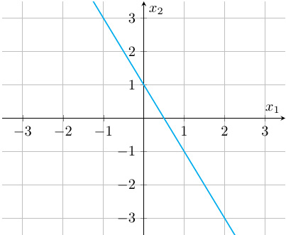
Figure 6.2 – The graph of the linear equation x2 = 1 – 2x1. Note that the line passes through points (x1, x2) = (1, -1) and (x1, x2) = (0, 1), which we can see clearly satisfy the equation

It turns out that the graph of every linear equation traces out a straight line in the Cartesian coordinate plane, which is precisely why we call them linear.

Definition – System of two linear equations in two variables

A linear system of two equations of variables x1 and x2 is made up of two linear equations of x1 and x2. A solution to the system is an ordered pair (x1, x2) that satisfies both equations simultaneously.

Since each equation can be represented as a line, the geometric equivalent of this problem is to find point(s) of intersection of the lines. Intuitively, it is clear two lines may cross at exactly one point, the lines may be parallel and never intersect, or the lines may coincide with one another entirely.

If the lines cross, we call the system consistent. If the lines are parallel, we call the system inconsistent. If the lines coincide, we call the system dependent. The next three examples will investigate each of these three situations.

Example – A consistent system

Consider the following system of two linear equations:

2x1 + 3x2 = -1

6x1 + 3x2 = 3

To find a solution to the system, we need to find coordinates x1 and x2 such that both equations are satisfied simultaneously. So, suppose these coordinates exist, then we can think about what must be true about them. The second equation must be true, so if we solve it for x2 (as we did earlier), we see x2 = -2x1 + 1, an expression of x2 in terms of x1. If we knew x1, this would provide a formula for us to establish the other coordinate, x2.

Since the first equation must also be satisfied for a solution (x1, x2), it must be valid to replace x2 with –2x1 + 1 in that equation, which provides a path to find x1:

2x1 + 3(-2x1 + 1) = -1.

Multiplying the 3 by each term in the parentheses, we have the following:

2x1 - 6x1 + 3 = -1.

Combining the x1 terms and subtracting 3 from each side of the equation, we have the following:

-4x1 = -4

This gives the value of x1 if we divide each side of the equation by -4:

x1 = 1

Thus, if there exists a solution, its x1 coordinate is 1, but we know we can compute x2 as

x2 = -2(1) + 1 = -2 + 1 = -1,

so, we see the solution must be (x1, x2) = (1, -1). Plotting the two lines on a graph confirms that the point (1, -1) is precisely where the two graphs of the linear equations cross:

Figure 6.3 – The graphs of the two linear equations cross at point (1, -1)

Since the lines cross at one point, it is a consistent system. The point (1, -1) is the only solution to the system of equations, the single point where the lines cross.

Example – An inconsistent system

Consider the following system of two linear equations:

2x1 + x2 = 3

6x1 + 3x2 = 3

To find a solution to the system, again, we need to find coordinates x1 and x2 such that both equations are satisfied simultaneously. So, suppose these coordinates exist, then we can think about what must be true about them. The second equation must be true, so if we solve it for x2 (as we did above), we see

x2 = -2x1 + 1,

an expression of x2 in terms of x1. If we knew x1, this would provide a formula for us to establish the other coordinate, x2.

Since the first equation must also be satisfied for a solution (x1, x2), it must be valid to replace x2 with –2x1 + 1 in that equation, which provides a path to find x1:

2x1 + (-2x1 + 1) = 3

Adding the x1 terms, we get

1 = 3.

Clearly something went wrong here, but what is it exactly? Our initial assumption was that there exists a point (x1, x2) that satisfies both equations, but this assumption logically implies a result that says 1 = 3, which is clearly false.

The proof by contradiction method we learned in Chapter 2, Formal Logic and Constructing Mathematical Proofs, reveals that this initial assumption must have been false, so there is no such point: there is no solution to this system of equations.

In the following graph, we see that the two lines are parallel, and therefore never cross one another. This means the lines share no points, as can be seen in the following graph:

Figure 6.4 – The graphs of the two linear equations in this example are parallel, so they never cross and there are no solutions to the system

As we defined previously, a linear system of equations that are geometrically represented as parallel lines is inconsistent. This means there is no solution to the system because there is no point that touches both lines.

Example – A dependent system

Consider the following system of two linear equations:

2x1 + x2 = 1

6x1 + 3x2 = 3

To find a solution to the system, again, we need to find coordinates x1 and x2 such that both equations are satisfied simultaneously. So, suppose these coordinates exist, then we can think about what must be true about them. The second equation must be true, so if we solve it for x2 (as we did previously), we see

x2 = -2x1 + 1,

an expression of x2 in terms of x1. If we knew x1, this would provide a formula for us to establish the other coordinate, x2.

Since the first equation must also be satisfied for a solution (x1, x2), it must be valid to replace x2 with –2x1 + 1 in that equation, which provides a path to find x1:

2x1 + (-2x1 + 1) = 1

Adding the x1 terms, we are left with only

1 = 1.

Once again, something does not seem quite right. Instead of getting the x1 coordinate we wanted, we get a simple result that says 1 = 1. This is obviously true, but it is not a solution to the linear system, so what does it mean?

If we take the second equation and divide it by 3, we get 2x1 + x2 = 1, the same as the first equation, so the second equation is not really adding any extra information in a sense. If a point (x1, x2) satisfies the first equation, of course it satisfies the second, and vice versa. Therefore, each line represents the same set of infinitely many points, so any point in the form (x1, -2x1 + 1), given a real number x1, is a solution.

We call such systems of linear equations with infinitely many solutions dependent because we have two equations representing identical lines, as can be seen in the following graph:

Figure 6.5 – The graphs of the two linear equations in this example are geometrically the same line, so every point on one line is on the other line, so they are all solutions to the system of equations

So far in this chapter, we have defined linear equations with two unknowns and drawn their graphs, which are lines. Then, we considered linear systems of two equations with two unknowns. As there are two linear equations, plotting the two equations results in two lines. Then, in a series of examples, we saw that there are three possible types of system of two linear equations:

• Consistent system: The lines cross at one point, which is the unique solution to the system.
• Inconsistent system: The lines never cross, so there are no solutions.
• Dependent system: The lines are the same, so all points on the line are solutions.

In the next couple of pages, we will extend these ideas to linear systems of more than two equations with more than two unknowns. Although the situation becomes more complicated in this setting, much of the preceding theory still applies. Linear systems are still classified the same way, with these same three classes.

Let's define a few more notions for these larger systems of linear equations before continuing to solve them, which turns out to be harder to do by hand than these examples, so we will turn to a number of Python functions to solve them for us once we understand the main idea of the solution method.

Definition – Systems of linear equations and their solutions

A system of n linear equations in variables x1, x2, …, xn is a set of equations in the following form:

where each aij and bi is a real constant. A solution to the system is a point (x1, x2, …, xn) in n-dimensional space that solves all of the equations simultaneously.

So, just like the definition when we limited it to two equations and two variables, we seek a point that solves all the equations. However, instead of the solution being a point in a 2D coordinate plane, the solutions to these are points in a higher dimensional space. The 3D case is easy to visualize, as we are accustomed to seeing the world in three dimensions, but it is not possible to visualize the higher dimensional spaces quite so well, so the geometric interpretations of solutions are not so easy to discuss. Nevertheless, the mathematics we will present produces accurate results in those higher dimensional spaces.

Definition – Consistent, inconsistent, and dependent systems

A system of n linear equations with n variables falls into one of three categories:

• If the system has one solution, it is called consistent.
• If the system has no solutions, it is called inconsistent.
• If the system has infinitely many solutions, it is called dependent.

It is possible to solve these larger systems of linear equations by hand by means of a substitution process similar to what we did in the preceding example, but it quickly gets very long and tedious, so we will present a standard method called Gaussian elimination that always works, but it is best left to algorithms in practice. However, we need to do some pre-processing to the system to put it into a special new form with some mathematical structures called matrices before we can use Gaussian elimination (both by hand and with Python).

Matrices and matrix representations of linear systems

Solving systems of more than two equations in more than two variables is very cumbersome under the algebraic notation we used previously for the small notations, so we need an alternate notation. We will take the coefficients of a system of n linear equations with n unknowns denoted aij above and arrange them in a special sort of array called a matrix. What makes matrices distinct from arrays you may be accustomed to using in code is that matrices have a special multiplication operation that simplifies many calculations and, especially, makes solving larger linear systems much easier.

We will also represent the xj and the bi terms as matrices to make a single matrix equation instead of n separate equations. Once we do that, we will be ready to solve these larger systems efficiently by hand and then with Python.

Definition – Matrices and vectors

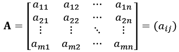
An m-by-n matrix A is a rectangular array of numbers with m rows and n columns, which have some associated mathematical operations defined between matrices and between numbers and matrices.

Each number in a matrix is called an entry or element of the matrix and the entry in the ith row and jth column is typically written with a lowercase aij. A matrix is usually written in the form

.

Vectors are matrices with either one row or one column. The following vectors are called the column vectors of A, where each column of A will become a vector:

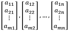
The following vectors are called the column vectors of A:

In Python, we can represent the following two matrices,

and ,

and access specific entries of the matrices in the following code:

import numpy

# initialize matrices

A = numpy.array([[3, 2, 1], [9, 0, 1], [3, 4, 1]])

B = numpy.array([[1, 1, 2], [8, 4, 1], [0, 0, 3]])

# print the entry in the first row and first column of A

print(A[0,0])

# print the entry in the second row and third column of B

print(B[1,2])

So, the code first creates the two matrices, A and B, given here. (They are called NumPy arrays in the language of Python.)

Then, we call and print the number in the very first row and very first column of matrix A, which in code is A[0,0], but in mathematical notation is a11 = 3, which the code outputs. Lastly, we similarly choose B[1,2], the element in row 2 and column 3 of matrix B, in other words, b23 = 1

3

1

It is important to be aware that Python and most other programming languages begin indexing arrays (and matrices) with 0 while mathematicians tend to start with 1, which is why the numbers in the code are one less than the mathematical language would suggest.

Important note

There is a matrix class built into NumPy that has been used for linear algebra, but current documentation says this class will be deprecated in the future, so users should use arrays instead. We will follow this convention.

Now that we have some common vocabulary about matrices, we will discuss ways to manipulate matrices, multiply them with numbers, add and subtract matrices, and multiply matrices. These operations are what distinguish matrices from ordinary arrays.

Definition – Matrix addition and subtraction

Let A = (aij) and B = (bij) be m-by-n matrices. Their sum is found by simply adding the entries of each matrix elementwise, meaning each aij is added to each bij as follows:

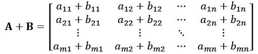
In other words, we add up the terms in the same positions in matrix A and in matrix B.

And the difference in two matrices works similarly, as can be seen here:

In other words, we subtract up the terms in the same positions in matrix A and in matrix B.

Important note

The sum and difference of two matrices is only defined if the two matrices have the same dimensions, in other words, the same number of rows and the same number of columns.

We can use the numpy.add and numpy.subtract functions to add and subtract matrices in Python as in the following code, which follows from the preceding code:

# Add A and B

print(numpy.add(A,B))

# Subtract A and B

print(numpy.subtract(A,B))

The code has the following output:

[[ 4  3  3]

[17  4  2]

[ 3  4  4]]

[[ 2  1 -1]

[ 1 -4  0]

[ 3  4 -2]]

Of course, this is in fact A + B and A – B, which we could find by hand if we add and subtract all the numbers in the matrices element by element.

Next, we continue with more arithmetic of matrices: multiplying a whole matrix by a scalar (or, by a number).

Definition – Scalar multiplication

Let c R be a real number. Such a constant is frequently referred to as a scalar. The product of this scalar c and a matrix A is defined as a matrix where each element is the product of c times the corresponding element of A:

In simpler terms, we simply take our real number c and multiply it by each and every number in the matrix.

As we see, the sum and differences of matrices and the scalar multiplication of matrices are somewhat obvious, as we simply do the operations for each element. Matrix multiplication, on the other hand, is not simply elementwise multiplication.

Before that, we define transposes of matrices and a special case of the matrix product called the dot product, which is limited to multiplying a row vector by a column vector.

Definition – Transpose of a matrix

Let A = (aij) be an m-by-n matrix. The transpose of A, denoted AT, is the n-by-m matrix resulting from switching each element in the ith row and jth column of A to the element in the jth row and ith column of the new matrix,

.

In simpler terms, a transpose moves the elements of a matrix around by swapping the row of an element with its column. Here are a couple of examples:

• Element a21 in row 2, column 1 of the original matrix A moves to row 1, column 2 in the new transpose matrix, AT.
• Element an1 in row n, column 1 of the original matrix A moves to row 1, column n in the new transpose matrix, AT.

  Important note

  The transpose of a matrix in general has different dimensions to the original matrix, with the number of rows and the number of columns interchanged.

We can also use NumPy to do scalar multiplication and find transposes, as the following code, continuing on from the previous code, will do:

# Multiply A by a scalar 5

print(numpy.multiply(5,A))

# Find the transpose of A

print(numpy.transpose(A))

The output of this code is as expected:

[[15 10  5]

[45  0  5]

[15 20  5]]

[[3 9 3]

[2 0 4]

[1 1 1]]

The first multiplication of 5 with the matrix A multiplies each element of the original matrix by the number 5. The second part takes a transpose properly by swapping the rows with the columns of the original A matrix.

To wrap up the section, we will look at multiplication not between a number and a matrix, but multiplication between two matrices, which has some special rules. This allows us to convert systems of linear equations of any size into a single matrix equation.

Definition – Dot product of vectors

The dot product of a 1-by-n row vector a and an n-by-1 column vector b is defined as

.

In other words, we multiply the first number in a by the first number in b, the second number in a by the second number in b, and so on, and add up all of the results of these multiplications.

In general, matrix multiplication for larger matrices computes dot products of the rows of the first matrix and columns of the second matrix.

Definition – Matrix multiplication

Let A be an n-by-m and let B be an m-by-p matrix, written in the forms

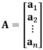and ,

where each ai and bj is a 1-by-m column vector. So, we represent our matrix A by stacking up its horizontal rows a1, a2, …, an, and we represent our matrix B by stacking its vertical columns side by side.

The product of the matrices is denoted by AB and the element of AB in the ith row and jth column is the dot product of the ith row of A and the jth column of B, as follows:

In simpler terms, matrix multiplication takes the dot product of each row vector of A with each column vector of B.

Important note

The matrix product AB is only defined when A has the same number of columns as B has rows, and AB has the same number of rows as A and the same number of columns as B. Thus, multiplying an n-by-m matrix by an m-by-p matrix is permitted and results in an n-by-p matrix.

This definition can feel a little difficult, so next, we will do an example where we carefully multiply two matrices by hand and then do it in Python.

Example – Multiplying matrices by hand and with NumPy

Define two matrices as

and .

Then, the product can be computed as

.

By the definition of matrix multiplication, this is a matrix made up of dot products of each row of A with each column of B:

To do each of the four dot products, we multiply the first term of a row by the first term of a column, the second term of a row by the second term of a column, and finally the third term in a row by the third term of a column and add them up:

Simplifying the arithmetic, we get

Suppose we were to multiply BA instead. This is possible since B is 3-by-2 and A is 2-by-3, so the result BA will be a 3-by-3 matrix. Unlike ordinary multiplication, with matrix multiplication, we have AB ≠ BA in some cases. Mathematically, this means matrix multiplication is not a commutative operation: the order of the factors matters.

We see matrix multiplication is easy enough to do by hand for a small matrix, but if the matrices were much larger, the number of steps in the arithmetic would make this pretty inefficient, so we generally prefer to use code. We may multiply matrices with NumPy with the following code. Again, this continues on from the previous code in this section:

# Multiply A and B

print(numpy.dot(A,B))

The output is as follows

[[19 11 11]

[ 9  9 21]

[35 19 13]]

Important note

NumPy has numpy.multiply and numpy.dot functions.

numpy.multiply performs component-wise multiplication.

numpy.dot performs matrix multiplication, as we defined previously.

Now that we know about matrix multiplication, the definition of a system of n linear equations with n unknowns x1, x2 …, xn can be written in terms of matrix multiplication as

,

which can be written much more compactly as Ax = b and we call it an n-by-n linear system, corresponding to the dimensions of A. Now, to see why this is true if things aren't clear, let's multiply out the matrix and see what happens. If we compute the dot product of row 1 of A by the x vector and set it equal to the top number in the b vector, we get

,

which is exactly the first equation in our system!

For another one, let's multiply the dot product row 2 of A by the x vector and set it equal to the second number in b:

,

which is the second equation in the system. Continuing this for each row, the matrix multiplication of A by x will generate each equation, one by one. So, we see this sort of matrix equation is equivalent to all n equations in our system, with each row corresponding to one of the equations.

Another common representation that we will use is a so-called augmented matrix to represent the system as follows:

.

Each row in the augmented matrix [A|b] corresponds to one of the equations. The ith row of [A|b] corresponds to the ith equation of the system:

ai1x1 + ai2x2 + … + ainxn = bi

Next, we look at an approach to solve these linear systems called Gaussian elimination and learn how to implement it with code.

Solving small linear systems with Gaussian elimination

In this section, we will learn how to solve an n-by-n linear system of equations Ax = b, if possible, through a method called Gaussian elimination, which we will do by hand for a small problem. In the next section, we implement it with Python.

We will explain through an example of a 3-by-3 system, which should make the idea clear for larger systems, which we will formalize at the end of the section, and which we will prefer to solve with code.

First, notice that there are several manipulations we may do to the equation in the system without changing the solutions:

• We can switch the order of the equations, which corresponds to swapping the rows of the matrix [A|b].
• We can multiply both sides of an equation by a constant, which corresponds to multiplying a row of [A|b] by a constant.
• We can add a multiple of one equation to another equation, which corresponds to adding a multiple of one row of [A|b] to another row.

The effects of the augmented matrix corresponding to each of these manipulations are called elementary row operations. Gaussian elimination is a method that will use specific sequences of row operations to manipulate the system into a very simple version that will make it immediately solvable or reveal it to be inconsistent or dependent. The form is shown next.

Definition – Leading coefficient (pivot)

For each row of a matrix not fully filled with zeros, the leading coefficient (or pivot) of the row is the first non-zero number in the row.

For example, consider the matrix

.

The pivots of this matrix are the 2 in the first row, the 1 in the second row, and the 5 in the third row.

Definition – Reduced row echelon form

A matrix is in reduced row echelon form (RREF) if the following applies:

• Any zero rows are on the bottom.
• The pivot of each non-zero row is a 1 and is to the right of the pivot of the previous row.
• Each column containing a 1 pivot has zeros in all other entries.

Example – Consistent system in RREF

For example, the following matrix is in RREF:

The corresponding linear system is simply

1x1 + 0x2 + 0x3 = 2

0x1 + 1x2 +0x3 = 3

0x1 + 0x2 + 1x3 = 1.

In other words, an augmented matrix in RREF immediately gives the solution of a linear system, (2, 3, 1) in this case, if it has a pivot in each row and we know the system is, therefore, consistent. In most cases, we will have a more complex augmented matrix initially that is transformed into this form using elementary row operations.

Example – Inconsistent system in RREF

Suppose a system has an augmented matrix in RREF as follows:

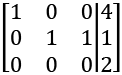
Even though the third column has multiple numbers in it, this is permitted since that column does not contain a pivot 1. The corresponding system of equations is

1x1 + 0x2 + 0x3 = 4

0x1 + 1x2 + 1x3 = 1

0x1 + 0x2 + 0x3 = 2.

However, the third row suggests 0 = 2, a contradictory statement. Just like the case with a system of two linear equations, this means the system is inconsistent – in other words, it has no solutions. In 2D, this means the lines are parallel, but in 3D, the equations represent planes, so it means at least two of the planes are parallel.

Example – Dependent system in RREF

Lastly, consider a system with the following RREF augmented matrix:

If we convert this RREF form back into equation form, we have

1x1 + 0x2 + 1x3 = 1

0x1 + 1x2 + 2x3 = 6

0x1 + 0x2 + 0x3 = 0.

The last line is true but tells us nothing about x3. Just like the 2D case, this means the system is dependent. In this situation, x3 is called a free variable because we can construct a point solving the system for any given x3 value.

Given x3, we know that x1 = 1 – x3 and x2 = 6 – 2x3, so the solution set for this system of three linear equations is {(1 – x3, 6 – 2x3, x3) : x3 R}, in other words, any ordered pair in this form is a solution.

Now we have learned the three permissible row operations and that we can easily determine the solution of a linear system if we have transformed the system's augmented matrix into RREF, so the question becomes, simply: Which row operations do we need to do to go from a given augmented matrix to RREF?

Gaussian elimination answers this question by providing a sequence of row operations that will never fail to do this conversion, which we define now.

Algorithm – Gaussian elimination

The specifics of different implementations of this method may vary and have some changes to optimize the calculations, but the most direct approach is provided by the following pseudocode:

Step 1: Re-order the rows of [A|b] from i to n so that the leftmost pivot is and pivots in subsequent rows are in the same column or to the right of the pivot of the previous row.

Step 2: Set i = 1.

Step 3: Divide row i by its pivot.

Step 4: Add multiples of row i to each successive row chosen such that the numbers under the pivot of row i become zeros.

Step 5: Add 1 to i.

Step 6: Move all zero rows of [A|b] to the bottom. Set m to be the number of zero rows.

Step 7: If i < n – m, return to Step 3. Otherwise, i = n – m and continue to Step 8.

Step 8: If row i has a pivot, add multiples of row i to all previous rows chosen such that the numbers above the pivot of row i become 0. Otherwise, proceed immediately to Step 9.

Step 9: Subtract 1 from i.

Step 10: If i = 1, terminate. Otherwise, return to Step 8.

The first phase of Gaussian elimination (Steps 1-6) ensures the matrix has all pivots set to 1 with 0s under them. The second phase (Steps 8-10) fills in 0s above the pivots so that the matrix is converted to RREF. Augmented matrices will represent the same linear system as the original [A|b].

Example – 3-by-3 linear system

Consider the system of linear equations:

2x1 – 6x2 + 6x3 = -8

2x1 + 3x2 – x3 = 15

4x1 – 3x2 – x3 = 10

We can write this system of equations as the following augmented matrix:

First, divide row 1 by 2 to get the following:

Next, add -2 times the first row to row 2 and -4 times the first row to row 3 to fill in zeros under the first pivot:

Then, divide row 2 by 9 so its pivot becomes 1:

Add -9 times row 2 to row 3:

Dividing row 3 by -6 completes the first phase of Gaussian elimination:

The remaining steps will comprise the second phase of Gaussian elimination. To fill in zeros above the last pivot, add 7/9 times row 3 to row 2 and add -3 times row 3 to row 1:

Lastly, add 3 times row 2 to row 1 to get to the RREF:

Thus, this RREF form reveals the system is consistent and its solution (5, 1, -2), is the numbers in the rightmost column.

In this section, we have introduced the reduced row echelon form (RREF) of a matrix corresponding to a linear system of equations introduced in the previous sections. The RREF always easily reveals the solution to the system if it exists, or reveals the system is inconsistent if there is no solution. After that, we considered an algorithm called Gaussian elimination that never to convert the matrix corresponding to an n-by-n linear system of equations to the RREF and, therefore, reveals the solution if possible. Lastly, we applied the algorithm by hand to a small, 3-by-3 linear system.

Now that we understand the problem Gaussian elimination solves and how it works, we will continue to learn how to implement the algorithm with NumPy.

Solving large linear systems with NumPy

The last example should make it clear that Gaussian elimination will work for any linear system to reduce it to RREF form, but this 3-equation, 3-variable system required a significant amount of effort to solve, and things will only become more complex for larger systems, so the more practical way to do it is to use existing algorithms. In this section, we will learn how to use some methods with NumPy to accomplish this task.

A Python function for solving systems of linear equations Ax = b is available in NumPy named numpy.linalg.solve, which works for square, consistent systems. That is, it finds solutions for all linear systems that have unique solutions.

Typically, the function uses a version of Gaussian elimination just as we have done by hand, but it is a very smart function. First, the function chooses the order of calculations carefully to optimize its speed. Second, if the function detects that A has a special structure (such as a symmetric, diagonal, or banded matrix), it will take shortcuts and use variants of Gaussian elimination and other methods that exploit the structure to run even faster!

Although we will not delve into these other methods since it would require an in-depth study of linear algebra, we can think of the function in terms of what it accomplishes and avoid the details. Nevertheless, we benefit from the speed-ups.

Let's try it!

Example – A 3-by-3 linear system (with NumPy)

We begin with a system we already solved by hand just to be sure we get the same answer from the NumPy function, so consider the linear system Ax = b with the augmented matrix form:

To solve this, we need to create two NumPy matrices, one for A and one for b to feed into the numpy.linalg.solve function and then run it:

import numpy

# Create A and b matrices

A = numpy.array([[2, -6, 6], [2, 3, -1], [4, -3, -1]])

b = numpy.array([-8, 15, 19])

# Solve Ax = b

numpy.linalg.solve(A,b)

The numpy.linalg.solve(A,b) line runs an optimized version of Gaussian elimination and code returns:

array([ 5.,  1., -2.])

In other words, the code tells us the solution is (5, 1, -2), just as we found by hand, but this time we get the solution almost instantaneously!

Example – Inconsistent and dependent systems with NumPy

We said numpy.linalg.solve requires consistent systems, but a reasonable question is what happens if you give it matrices A and b corresponding to an inconsistent or dependent system, so let's try the inconsistent and dependent systems we considered in the first example of the chapter.

In the following code, we repeat the same idea as the previous example twice more, but this time, we solve the inconsistent and dependent problems we solved before:

import numpy

# inconsistent system

A = numpy.array([[2, 1], [6, 3]])

b = numpy.array([3, 3])

print(numpy.linalg.solve(A,b))

# dependent system

A = numpy.array([[2, 1], [6, 3]])

b = numpy.array([1, 3])

print(numpy.linalg.solve(A,b))

The output is as follows:

[-1.80143985e+16  3.60287970e+16]

[0. 1.]

For the inconsistent system, it returns some giant numbers in the order of 1016, but we know there is no solution mathematically, so this is meaningless. In the case of the dependent system, it returns (0, 1), which is a solution to the system, but it has infinitely many solutions.

A key take-away from this example is that we should never implement numpy.linalg.solve without carefully screening the coefficient matrix A we will feed into it because it will return nonsense or incomplete answers without giving us any sort of warning.

How can we test A? The theory required is beyond the scope of this book, but there is a number called a determinant that can be computed for a square matrix and there is a theorem called the Invertible Matrix Theorem that tells us a linear system is always consistent if the determinant of A is not 0. Therefore, a good practice is to verify that the determinant of A is nonzero with the numpy.linalg.det function before proceeding further. In the following code, we create a NumPy array A, compute the determinant, and print it:

A = numpy.array([[2, 1], [6, 3]])

print(numpy.linalg.det(A))

This produces the following output:

-3.330669073875464e-16

This is a number in the order of 10-16, which is extremely tiny and suggests the determinant is effectively 0, which would indicate numpy.linalg.solve should not be used. In a practical implementation, we would want to check this first and output an error if the determinant is within 10-5 of 0 in order to account for rounding errors.

Where the numpy.linalg.solve method really shines is in larger linear systems of equations, which would be totally unreasonable to do by hand. The 3-by-3 linear system took a whole 2 pages to solve with Gaussian elimination. It would be almost unthinkable to solve a system of 10, 20, or 100 equations by hand! It turns out, however, that these are not difficult for NumPy.

Example – A 10-by-10 linear system (with NumPy)

It would be cumbersome to even write down a 10-by-10 linear system of equations, so we will rely on the short expression Ax = b, but which system will we solve? To save the trouble of making up a problem, suppose we just generate matrices A and b with uniformly random numbers.

It requires some deep mathematics beyond the scope of this book, but it can be shown such a system is consistent with probability 1, so it is highly likely to satisfy the requirements for numpy.linalg.solve():

The following code will do three primary things:

• Generate A and b as 10-by-10 and 10-by-1 matrices, respectively, with elements selected uniformly at random from the interval [-5, 5] using numpy.random.rand.
• Use numpy.linalg.solve to find a 10-by-1 matrix x that solves the system, and then calculates Ax – b using numpy.dot for the multiplication.
• Sum the absolute values of the 10-by-1 matrix Ax – b to verify the result is nearly 0, possibly with some tiny error resulting from rounding errors, to confirm the solution is correct:

  import numpy

  numpy.random.seed(1)

  # Create A and b matrices with random

  A = 10*numpy.random.rand(10,10)-5

  b = 10*numpy.random.rand(10)-5

  # Solve Ax = b

  solution = numpy.linalg.solve(A,b)

  print(solution)

  # To verify the solution works, show Ax - b is near 0

  sum(abs(numpy.dot(A,solution) - b))

  This returns the following output:

  [ 0.09118027 -1.51451319 -2.48186344 -2.94076307  

    0.07912968  2.76425416 2.48851394 -0.30974375   

      -1.97943716 0.75619575]

  1.1546319456101628e-14

As you can see, numpy.linalg.solve(A,b) finds that the solution to this 10-by-10 system of linear equations is roughly (0.09, -1.51, -2.48, -2.94, 0.08, 2.76, 2.49, -0.31, -1.98, 0.76).

Note that sum and abs are some common Python function for adding and finding the absolute values of elements of a matrix. The last line of code sums the absolute values of Ax – b to get a number of nearly 0. This tells us Ax – b is approximately 0, so we have confirmation that the solution is accurate, at least to 14 decimal places.

Important note

The numpy.random.seed(1) command is used simply so that the code is reproducible for readers.

If you remove this line, the calls to numpy.random.rand will generate different random numbers so that it generates a different 10-by-10 linear system of equations and solves it.

This is a good practice for testing code with randomness.

Once again, this code runs almost instantaneously on a typical laptop, even though it solves a rather large system by the standards of what we can compute by hand. In fact, the performance of this function is truly extraordinary: it runs almost instantaneously even if we replace a 10-by-10 system with a 1,000-by-1,000 system. Indeed, it solves a linear system of 1,000 equations with 1,000 variables with sums of absolute errors in the order of 10-10 in almost no time!

Summary

In this chapter, we covered a lot of ground! We began by taking the familiar idea of a linear equation in two variables and demonstrated that the set of points that satisfy the equation are exactly those that form a straight line. We then extended this to a system of two linear equations of two variables, which represent, geometrically speaking, two lines. A solution to the system is a point that satisfies not one, but both equations. Geometrically, this means a solution can only be a point of intersection of the two lines. As we know from elementary geometry, two lines must either be parallel, intersect, or coincide entirely. This characterizes three possible conclusions about solutions: a system must have no solutions (if they are parallel), one unique solution (if they intersect), or infinitely many solutions (if they coincide).

Then, the real fun started as we introduced systems of many linear equations and many unknowns, which are not so easily interpretable from a geometrical perspective, but they share this same property, that there must be zero, one, or infinitely many solutions.

We found these larger problems to be very cumbersome to solve with basic algebra, so we introduced a new mathematical structure to tackle this problem more efficiently: the matrix. We learned matrices behave similar to an ordinary rectangular array of numbers, but there is a special notion of multiplication of matrices that allows us to represent even large linear systems of equations in a compact, rectangular form that makes computation efficient.

After learning how to perform these matrix operations using NumPy functions, we proceeded to solve larger linear systems of equations. We learned an efficient method called Gaussian elimination that solves these systems, solved an example system of three linear equations with three variables, and then proceeded to learn to use NumPy's implementation of optimized Gaussian elimination in Python.

As we proceed through the remaining chapters, we will actually be using these methods very frequently, as linear algebra is critical for a wide array of applied problems that we will study, ranging from problems on trees and networks, cryptography, and regression analysis, to image processing and principal component analysis.

The next chapter is the first in a sequence of chapters based on tree, graph, and network structures, which are incredibly important for modeling many things, such as decision trees that guide helpdesk workers through best practices, linking structures of the web, and computer networks. In this next chapter, we define these structures, learn what they commonly model, use Python to store them efficiently, learn how to use linear algebra to find some features of the structures, and examine some key mathematical results in the area of graph theory with implications for computer science.