
Basic Electronic Circuit Components
3.1 Wires, Cables, and Connectors
Wires and cables provide low-resistance pathways for electric currents. Most electrical wires are made from copper or silver and typically are protected by an insulating coating of plastic, rubber, or lacquer. Cables consist of a number of individually insulated wires bound together to form a multiconductor transmission line. Connectors, such as plugs, jacks, and adapters, are used as mating fasteners to join wires and cable with other electrical devices.
3.1.1 Wires
A wire’s diameter is expressed in terms of a gauge number. The gauge system, as it turns out, goes against common sense. In the gauge system, as a wire’s diameter increases, the gauge number decreases. At the same time, the resistance of the wire decreases. When currents are expected to be large, smaller-gauge wires (large-diameter wires) should be used. If too much current is sent through a large-gauge wire (small-diameter wire), the wire could become hot enough to melt. Table 3.1 shows various characteristics for B&S-gauged copper wire at 20°C. For rubber-insulated wire, the allowable current should be reduced by 30 percent.
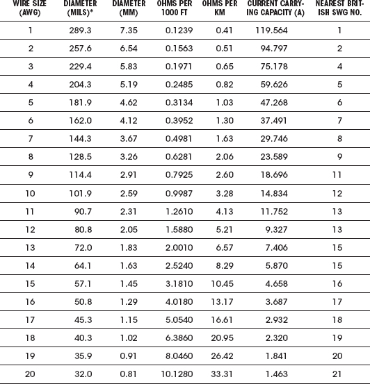
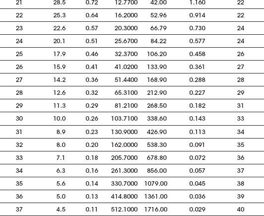
* 1 Mil = 2.54 × 10⁻⁵ m
Wire comes in solid core, stranded, or braided forms.
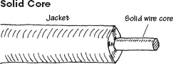
This wire is useful for wiring breadboards; the solid-core ends slip easily into breadboard sockets and will not fray in the process. These wires have the tendency to snap after a number of flexes.
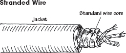
The main conductor is comprised of a number of individual strands of copper. Stranded wire tends to be a better conductor than solid-core wire because the individual wires together comprise a greater surface area. Stranded wire will not break easily when flexed.
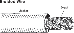
A braided wire is made up of a number of individual strands of wire braided together. Like stranded wires, these wires are better conductors than solid-core wires, and they will not break easily when flexed. Braided wires are frequently used as an electromagnetic shield in noise-reduction cables and also may act as a wire conductor within the cable (e.g., coaxial cable).
FIGURE 3.1
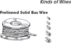
This wire is often referred to as hookup wire. It includes a tin-lead alloy to enhance solderability and is usually insulated with polyvinyl chloride (PVC), polyethylene, or Teflon. Used for hobby projects, preparing printed circuit boards, and other applications where small bare-ended wires are needed.
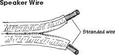
This wire is stranded to increase surface area for current flow. It has a high copper content for better conduction.
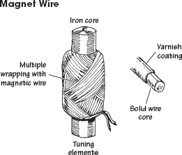
This wire is used for building coils and electromagnets or anything that requires a large number of loops, say, a tuning element in a radio receiver. It is built of solid-core wire and insulated by a varnish coating. Typical wire sizes run from 22 to 30 gauge.
FIGURE 3.2
3.1.2 Cables
A cable consists of a multiple number of independent conductive wires. The wires within cables may be solid core, stranded, braided, or some combination in between. Typical wire configurations within cables include the following:
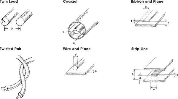
FIGURE 3.3
3.1.3 Connectors
The following is a list of common plug and jack combinations used to fasten wires and cables to electrical devices. Connectors consist of plugs (male-ended) and jacks (female-ended). To join dissimilar connectors together, an adapter can be used.

This cable is made from two individually insulated conductors. Often it is used in dc or low-frequency ac applications.

This cable is composed of two interwound insulated wires. It is similar to a paired cable, but the wires are held together by a twist.
The common CAT5 cable used for Ethernet, among other things, is based on a set of four twisted pairs.

This cable is a flat two-wire line, often referred to as 300-Ω line. The line maintains an impedance of 300 Ω. It is used primarily as a transmission line between an antenna and a receiver (e.g., TV, radio). Each wire within the cable is stranded to reduce skin effects.
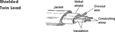
This cable is similar to paired cable, but the inner wires are surrounded by a metal-foil wrapping that’s connected to a ground wire. The metal foil is designed to shield the inner wires from external magnetic fields—potential forces that can create noisy signals within the inner wires.
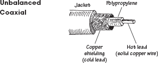
This cable typically is used to transport high-frequency signals (e.g., radio frequencies). The cable’s geometry limits inductive and capacitive effects and also limits external magnetic interference. The center wire is made of solid-core copper or aluminium wire and acts as the hot lead. An insulative material, such as polyethylene, surrounds the center wire and acts to separate the center wire from a surrounding braided wire. The braided wire, or copper shielding, acts as the cold lead or ground lead. Characteristic impedances range from about 50 to 100 Ω.
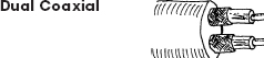
This cable consists of two unbalanced coaxial cables in one. It is used when two signals must be transferred independently.
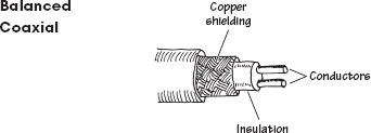
This cable consists of two solid wires insulated from one another by a plastic insulator. Like unbalanced coaxial cable, it too has a copper shielding to reduce noise pickup. Unlike unbalanced coaxial cable, the shielding does not act as one of the conductive paths; it only acts as a shield against external magnetic interference.

This type of cable is used in applications where many wires are needed. It tends to flex easily. It is designed to handle low-level voltages and often is found in digital systems, such as computers, to transmit parallel bits of information from one digital device to another.
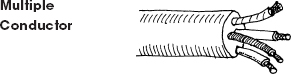
This type of cable consists of a number of individually wrapped, color-coded wires. It is used when a number of signals must be sent through one cable.
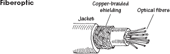
Fiberoptic cable is used in the transport of electromagnetic signals, such as light. The conducting-core medium is made from a glass material surrounded by a fiberoptic cladding (a glass material with a higher index of refraction than the core). An electromagnetic signal propagates down the cable by multiple total internal reflections. It is used in direct transmission of images and illumination and as waveguides for modulated signals used in telecommunications. One cable typically consists of a number of individual fibers.
FIGURE 3.4
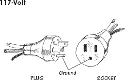
This is a typical home appliance connector. It comes in unpolarized and polarized forms. Both forms may come with or without a ground wire.
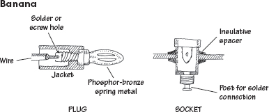
This is used for connecting single wires to electrical equipment. It is frequently used with testing equipment. The plug is made from a four-leafed spring tip that snaps into the jack.
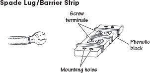
This is a simple connector that uses a screw to fasten a metal spade to a terminal. A barrier strip often acts as the receiver of the spade lugs.
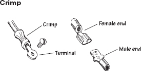
Crimp connectors are color-coded according to the wire size they can accommodate. They are useful as quick, friction-type connections in dc applications where connections are broken repeatedly. A crimping tool is used to fasten the wire to the connector.
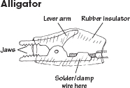
Alligator connectors are used primarily as temporary test leads.
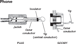
These connectors accept shielded braid, but they are larger in size. They come in two-or three-element types and have a barrel that is 1¼ in (31.8 mm) long. They are used as connectors in microphone cables and for other low-voltage, low-current applications.
3.5 mm and even 2.5 mm versions of these connectors are also commonly used.
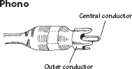
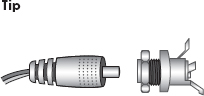
Phono connectors are often referred to as RCA plugs or pin plugs. They are used primarily in audio connections.
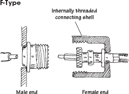
F-type connectors are used with a variety of unbalanced coaxial cables. They are commonly used to interconnect video components. F-type connectors are either threaded or friction-fit together.
These connectors are commonly used to supply low voltage dc between 3 and 15V.

IDC connectors are often found in computers. The plug is attached to ribbon cable using v-shaped teeth that are squeezed into the cable insulation to make a solderless contact.
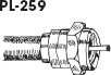
These are often referred to as UHF plugs. They are used with RG-59/U coaxial cable. Such connectors may be threaded or friction-fit together.
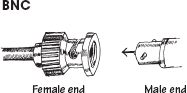
BNC connectors are used with coaxial cables. Unlike the F-type plug, BNC connectors use a twist-on bayonet-like locking mechanism. This feature allows for quick connections
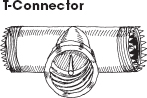
T-connectors consist of two plug ends and one central jack end. They are used when a connection must be made somewhere along a coaxial cable.
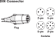
These connectors are used with multiple conductor wires. They are often used for interconnecting audio and computer accessories.
Smaller versions of these connectors (mini-DIN) are also widely used.
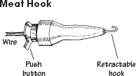
These connectors are used as test probes. The spring-loaded hook opens and closes with the push of a button. The hook can be clamped onto wires and component leads.
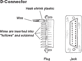
D-connectors are used with ribbon cable. Each connector may have as many as 50 contacts. The connection of each individual wire to each individual plug pin or jack socket is made by sliding the wire in a hollow metal collar at the backside of each connector. The wire is then soldered into place.
FIGURE 3.5
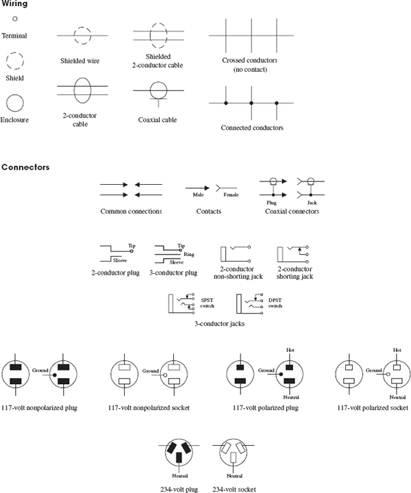
FIGURE 3.6
Weird Behavior in Wires (Skin Effect)
When dealing with low-current dc hobby projects, wires and cables are straightforward—they act as simple conductors with essentially zero resistance. However, when you replace dc currents with very high-frequency ac currents, weird things begin to take place within wires. As you will see, these “weird things” will not allow you to treat wires as perfect conductors.
First, let’s take a look at what is going on in a wire when a dc current is flowing through it.
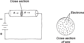
A wire that is connected to a dc source will cause electrons to flow through the wire in a manner similar to the way water flows through a pipe. This means that the path of any one electron essentially can be anywhere within the volume of the wire (e.g., center, middle radius, surface).
FIGURE 3.7
Now, let’s take a look at what happens when a high-frequency ac current is sent through a wire.
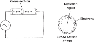
An ac voltage applied across a wire will cause electrons to vibrate back and forth. In the vibrating process, the electrons will generate magnetic fields. By applying some physical principles (finding the forces on every electron that result from summing up the individual magnetic forces produced by each electron), you find that electrons are pushed toward the surface of the wire. As the frequency of the applied signal increases, the electrons are pushed further away from the center and toward the surface. In the process, the center region of the wire becomes devoid of conducting electrons.
FIGURE 3.8
The movement of electrons toward the surface of a wire under high-frequency conditions is called the skin effect. At low frequencies, the skin effect does not have a large effect on the conductivity (or resistance) of the wire. However, as the frequency increases, the resistance of the wire may become an influential factor. Table 3.2 shows just how influential skin effect can be as the frequency of the signal increases (the table uses the ratio of ac resistance to dc resistance as a function of frequency).
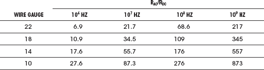
One thing that can be done to reduce the resistance caused by skin effects is to use stranded wire—the combined surface area of all the individual wires within the conductor is greater than the surface area for a solid-core wire of the same diameter.
Weird Behavior in Cables (Lecture on Transmission Lines)
Like wires, cables also exhibit skin effects. In addition, cables exhibit inductive and capacitive effects that result from the existence of magnetic and electrical fields within the cable. A magnetic field produced by the current through one wire will induce a current in another. Likewise, if two wires within a cable have a net difference in charge between them, an electrical field will exist, thus giving rise to a capacitive effect.
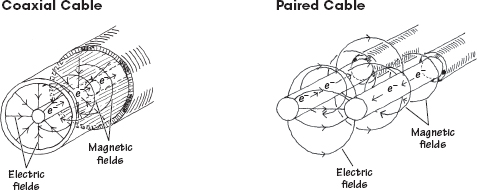
FIGURE 3.9 Illustration of the electrical and magnetic fields within a coaxial and paired cable.
Taking note of both inductive and capacitive effects, it is possible to treat a cable as if it were made from a number of small inductors and capacitors connected together. An equivalent inductor-capacitor network used to model a cable is shown in Fig. 3.10.
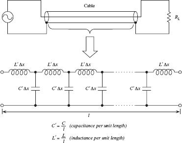
The impedance of a cable can be modeled by treating it as a network of inductors and capacitors.
FIGURE 3.10
To simplify this circuit, we apply a reduction trick; we treat the line as an infinite ladder and then assume that adding one “rung” to the ladder (one inductor-capacitor section to the system) will not change the overall impedance Z of the cable. What this means—mathematically speaking—is we can set up an equation such that Z = Z + (LC section). This equation can then be solved for Z. After that, we find the limit as Δx goes to zero. The mathematical trick and the simplified circuit are shown below.
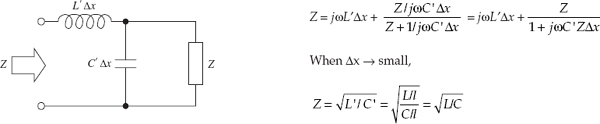
FIGURE 3.11
By convention, the impedance of a cable is called the characteristic impedance (symbolized Z0). Notice that the characteristic impedance Z0 is a real number. This means that the line behaves like a resistor despite the fact that we assumed the cable had only inductance and capacitance built in.
The question remains, however, what are L and C? Well, figuring out what L and C should be depends on the particular geometry of the wires within a cable and on the type of dielectrics used to insulate the wires. You could find L and C by applying some physics principles, but instead, let’s cheat and look at the answers. The following are the expressions for L and C and Z0 for both a coaxial and parallel-wire cable:
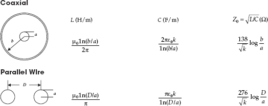
FIGURE 3.12 Inductance, capacitance, and characteristic impedance formulas for coaxial and parallel wires.
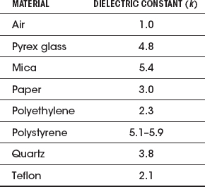
Here, k is the dielectric constant of the insulator, μ0 = 1.256 × 10⁻⁶ H/m is the permeability of free space, and ε0 = 8.85 × 10⁻¹² F/m is the permitivity of free space. Table 3.3 provides some common dielectric materials with their corresponding constants.
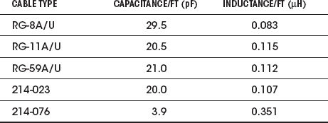
Often, cable manufacturers supply capacitance per foot and inductance per foot values for their cables. In this case, you can simply plug the given manufacturer’s values into  to find the characteristic impedance of the cable. Table 3.4 shows capacitance per foot and inductance per foot values for some common cable types.
TABLE 3.4 Capacitance and Inductance per Foot for Some Common Transmission-Line Types
Sample Problems (Finding the Characteristic Impedance of a Cable)
EXAMPLE 1
An RG-11AU cable has a capacitance of 21.0 pF/ft and an inductance of 0.112 μH/ft. What is the characteristic impedance of the cable?
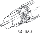
You are given the capacitance and inductance per unit length: C′ = C/ft, L′ = L/ft. Using  and substituting C and L into it, you get
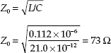
FIGURE 3.13
EXAMPLE 2
What is the characteristic impedance of the RG-58/U coaxial cable with polyethylene dielectric (k = 2.3) shown below?
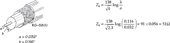
FIGURE 3.14
Find the characteristic impedance of the parallel-wire cable insulated with polyethylene (k = 2.3) shown below.
FIGURE 3.15
Impedance Matching
Since a transmission line has impedance built in, the natural question to ask is, How does the impedance affect signals that are relayed through a transmission line from one device to another? The answer to this question ultimately depends on the impedances of the devices to which the transmission line is attached. If the impedance of the transmission line is not the same as the impedance of, say, a load connected to it, the signals propagating through the line will only be partially absorbed by the load. The rest of the signal will be reflected back in the direction it came. Reflected signals are generally bad things in electronics. They represent an inefficient power transfer between two electrical devices. How do you get rid of the reflections? You apply a technique called impedance matching. The goal of impedance matching is to make the impedances of two devices—that are to be joined—equal. The impedance-matching techniques make use of special matching networks that are inserted between the devices.
Before looking at the specific methods used to match impedances, let’s first take a look at an analogy that should shed some light on why unmatched impedances result in reflected signals and inefficient power transfers. In this analogy, pretend that the transmission line is a rope that has a density that is analogous to the transmission line’s characteristic impedance Z0. Pretend also that the load is a rope that has a density that is analogous to the load’s impedance ZL. The rest of the analogy is carried out below.
Unmatched Impedances (Z0 < ZL)
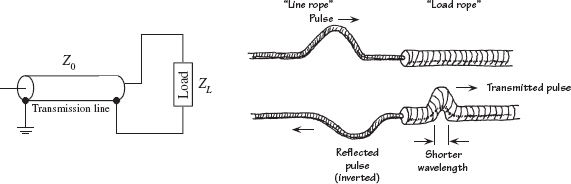
FIGURE 3.16a
A low-impedance transmission line that is connected to a high-impedance load is analogous to a low-density rope connected to a high-density rope. In the rope analogy, if you impart a pulse at the left end of the low-density rope (analogous to sending an electrical signal through a line to a load), the pulse will travel along without problems until it reaches the high-density rope (load). According to the laws of physics, when the wave reaches the high-density rope, it will do two things. First, it will induce a smaller-wavelength pulse within the high-density rope, and second, it will induce a similar-wavelength but inverted and diminished pulse that rebounds back toward the left end of the low-density rope. From the analogy, notice that only part of the signal energy from the low-density rope is transmitted to the high-density rope. From this analogy, you can infer that in the electrical case similar effects will occur—only now you are dealing with voltage and currents and transmission lines and loads.
Unmatched Impedances (Z0 > ZL)
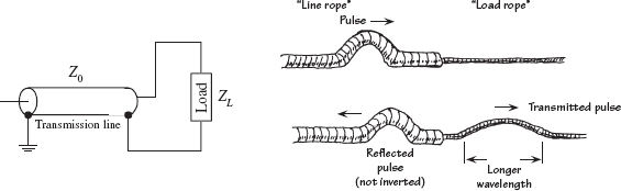
FIGURE 3.16b
A high-impedance transmission line that is connected to a low-impedance load is analogous to a high-density rope connected to a low-density rope. If you impart a pulse at the left end of the high-density rope (analogous to sending an electrical signal through a line to a load), the pulse will travel along the rope without problems until it reaches the low-density rope (load). At that time, the pulse will induce a longer-wavelength pulse within the low-density rope and will induce a similar-wavelength but inverted and diminished pulse that rebounds back toward the left end of the high-density rope. From this analogy, again you can see that only part of the signal energy from the high-density rope is transmitted to the low-density rope.
Matched Impedances (Z0 = ZL)
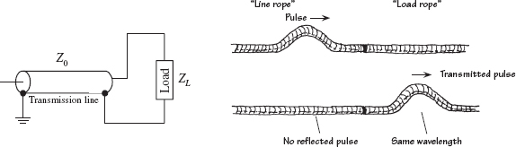
FIGURE 3.16c
Connecting a transmission line and load of equal impedances together is analogous to connecting two ropes of similar densities together. When you impart a pulse in the “transmission line” rope, the pulse will travel along without problems. However, unlike the first two analogies, when the pulse meets the load rope, it will continue on through the load rope. In the process, there will be no reflection, wavelength change, or amplitude change. From this analogy, you can infer that if the impedance of a transmission line matches the impedance of the load, power transfer will be smooth and efficient.
Standing Waves
Let’s now consider what happens to an improperly matched line and load when the signal source is producing a continuous series of sine waves. You can, of course, expect reflections as before, but you also will notice that a superimposed standing-wave pattern is created within the line. The standing-wave pattern results from the interaction of forward-going and reflected signals. Figure 3.17 shows a typical resulting standing-wave pattern for an improperly matched transmission line attached between a sinusoidal transmitter and a load. The standing-wave pattern is graphed in terms of amplitude (expressed in terms of Vrms) versus position along the transmission line.
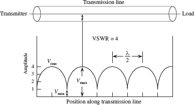
FIGURE 3.17 Standing waves on an improperly terminated transmission line. The VSWR is equal to Vmax/Vmin.
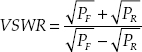
A term used to describe the standing-wave pattern is the voltage standing-wave ratio (VSWR). The VSWR is the ratio between the maximum and minimum rms voltages along a transmission line and is expressed as
The standing-wave pattern shown in Fig. 3.17 has VSWR of 4/1, or 4.
Assuming that the standing waves are due entirely to a mismatch between load impedance and characteristic impedance of the line, the VSWR is simply given by either
whichever produces a result that is greater than 1.
A VSWR equal to 1 means that the line is properly terminated, and there will be no reflected waves. However, if the VSWR is large, this means that the line is not properly terminated (e.g., a line with little or no impedance attached to either a short or open circuit), and hence there will be major reflections.
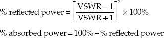
To make this expression meaningful, you can convert it into an expression in terms of forward and reflected power. In the conversion, you use P = IV = V2/R. Taking P to be proportional to V2, you can rewrite the VSWR in terms of forward and reflected power as follows:
Rearranging this equation, you get the percentage of reflected power and percentage of absorbed power in terms of VSWR:
EXAMPLE (VSWR)
Find the standing-wave ratio (VSWR) of a 50-Ω line used to feed a 200-Ω load. Also find the percentage of power that is reflected at the load and the percentage of power absorbed by the load.
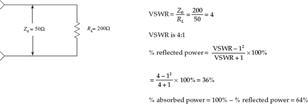
FIGURE 3.18
Techniques for Matching Impedances
This section looks at a few impedance-matching techniques. As a rule of thumb, with most low-frequency applications where the signal’s wavelength is much larger than the cable length, there is no need to match line impedances. Matching impedances is usually reserved for high-frequency applications. Moreover, most electrical equipment, such as oscilloscopes, video equipment, etc., has input and output impedances that match the characteristic impedances of coaxial cables (typically 50 Ω). Other devices, such as television antenna inputs, have characteristic input impedances that match the characteristic impedance of twin-lead cables (300 Ω). In such cases, the impedance matching is already taken care of.
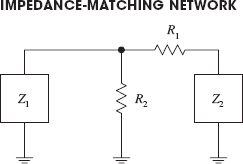
A general method used to match impedance makes use of the impedance-matching network shown here. To match impedances, choose
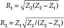
The attenuation seen from the Z1 end will be A1 = R1/Z2 + 1. The attenuation seen from the Z2 end will be A2 = R1/R2 + R1/Z1 + 1.
For example, if Z1 = 50 W, and Z2 = 125 W, then R1, R2, A1, and A2 are
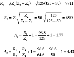
FIGURE 3.19
Here, a transformer is used to match the characteristic impedance of a cable with the impedance of a load. By using the formula
you can match impedances by choosing appropriate values for NP and NS so that the ratio NP/NS is equal to  .
.
For example, if you wish to match an 800-Ω impedance line with an 8-Ω load, you first calculate
To match impedances, you select NP (number of coils in the primary) and NS (number of coils in the secondary) in such a way that NP/NS = 10. One way of doing this would be to set NP equal to 10 and NS equal to 1. You also could choose NP equal to 20 and NS equal to 2 and you would get the same result.
FIGURE 3.20
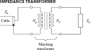
A broadband transmission-line transformer is a simple device that consists of a few turns of miniature coaxial cable or twisted-pair cable wound about a ferrite core. Unlike conventional transformers, this device can more readily handle high-frequency matching (its geometry eliminates capacitive and inductive resonance behavior). These devices can handle various impedance transformations and can do so with incredibly good broadband performance (less than 1 dB loss from 0.1 to 500 MHz).
FIGURE 3.21
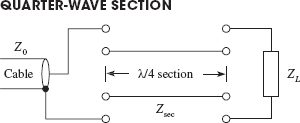
FIGURE 3.22
A transmission line with characteristic impedance Z0 can be matched with a load with impedance ZL by inserting a wire segment that has a length equal to one quarter of the transmitted signal’s wavelength (λ/4) and which has an impedance equal to
To calculate the segment’s length, you must use the formula λ = v/f, where v is the velocity of propagation of a signal along the cable and f is the frequency of the signal. To find v, use
where c = 3.0 × 10⁸ m/s, and k is the dielectric constant of the cable’s insulation.
For example, say you wish to match a 50-Ω cable that has a dielectric constant of 1 with a 200-Ω load. If you assume the signal’s frequency is 100 MHz, the wavelength then becomes
To find the segment length, you plug λ into λ/4. Hence the segment should be 0.75 m long. The wire segment also must have an impedance equal to
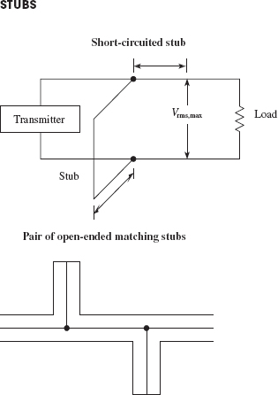
A short length of transmission line that is open ended or short-circuit terminated possesses the property of having an impedance that is reactive. By properly choosing a segment of open-circuit or short-circuit line and placing it in shunt with the original transmission line at an appropriate position along the line, standing waves can be eliminated. The short segment of wire is referred to as a stub. Stubs are made from the same type of cable found in the transmission line. Figuring out the length of a stub and where it should be placed is fairly tricky. In practice, graphs and a few formulas are required. A detailed handbook on electronics is the best place to learn more about using stubs.
FIGURE 3.23
3.2 Batteries
A battery is made up of a number of cells. Each cell contains a positive terminal, or cathode, and a negative terminal, or anode. (Note that most other devices treat anodes as positive terminals and cathodes as negative terminals.)
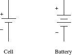
FIGURE 3.24
When a load is placed between a cell’s terminals, a conductive bridge is formed that initiates chemical reactions within the cell. These reactions produce electrons in the anode material and remove electrons from the cathode material. As a result, a potential is created across the terminals of the cell, and electrons from the anode flow through the load (doing work in the process) and into the cathode.
A typical cell maintains about 1.5 V across its terminals and is capable of delivering a specific amount of current that depends on the size and chemical makeup of the cell. If more voltage or power is needed, a number of cells can be added together in either series or parallel configurations. By adding cells in series, a larger-voltage battery can be made, whereas adding cells in parallel results in a battery with a higher current-output capacity. Figure 3.25 shows a few cell arrangements.
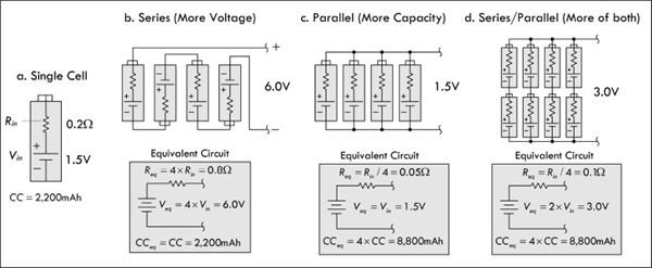
FIGURE 3.25
Battery cells are made from a number of different chemical ingredients. The use of a particular set of ingredients has practical consequences on the battery’s overall performance. For example, some cells are designed to provide high open-circuit voltages, whereas others are designed to provide large current capacities. Certain kinds of cells are designed for light-current, intermittent applications, whereas others are designed for heavy-current, continuous-use applications. Some cells are designed for pulsing applications, where a large burst of current is needed for a short period of time. Some cells have good shelf lives; others have poor shelf lives. Batteries that are designed for one-time use, such as carbon-zinc and alkaline batteries, are called primary batteries. Batteries that can be recharged a number of times, such as nickel metal hydride and lead-acid batteries, are referred to as secondary batteries.
3.2.1 How a Cell Works
A cell converts chemical energy into electrical energy by going through what are called oxidation-reduction reactions (reactions that involve the exchange of electrons). The three fundamental ingredients of a cell used to initiate these reactions include two chemically dissimilar metals (positive and negative electrodes) and an electrolyte (typically a liquid or pastelike material that contains freely floating ions). The following is a little lecture on how a simple lead-acid battery works.
For a lead-acid cell, one of the electrodes is made from pure lead (Pb); the other electrode is made from lead oxide (PbO2); and the electrolyte is made from a sulfuric acid solution (H2O + H2SO4 → 3H+ + SO42− + OH−).
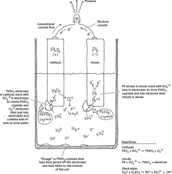
FIGURE 3.26
When the two chemically dissimilar electrodes are placed in the sulfuric acid solution, the electrodes react with the acid (SO4−2, H+ ions), causing the pure lead electrode to slowly transform into PbSO4 crystals. During this transformation reaction, two electrons are liberated within the lead electrode. Now, if you examine the lead oxide electrode, you also will see that it too is converted into PbSO4 crystals. However, instead of releasing electrons during its transformation, it releases O22− ions. These ions leak out into the electrolyte solution and combine with the hydrogen ions to form H2O (water). By placing a load element, say, a lightbulb, across the electrodes, electrons will flow from the electron-abundant lead electrode, through the bulb’s filament, and into the electron-deficient lead oxide electrode.
As time passes, the ingredients for the chemical reactions run out (the battery is drained). To get energy back into the cell, a reverse voltage can be applied across the cell’s terminals, thus forcing the reactions backward. In theory, a lead-acid battery can be drained and recharged indefinitely. However, over time, chunks of crystals will break off from the electrodes and fall to the bottom of the container, where they are not recoverable. Other problems arise from loss of electrolyte due to gasing during electrolysis (a result of overcharging) and due to evaporation.
3.2.2 Primary Batteries
Primary batteries are one-shot deals—once they are drained, it is all over. Common primary batteries include carbon-zinc batteries, alkaline batteries, mercury batteries, silver oxide batteries, zinc air batteries, and silver-zinc batteries. Here are some common battery packages:
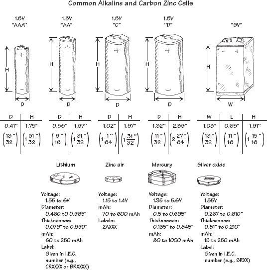
FIGURE 3.27
Carbon-Zinc Batteries
Carbon-zinc batteries (“standard-duty”) are general-purpose primary-type batteries that were popular back in the 1970s, but have become obsolete with the advent of alkaline batteries. These batteries are not suitable for continuous use (only for intermittent use) and are susceptible to leakage. The nominal voltage of a carbon-zinc cell is about 1.5 V, but this value gradually drops during service. Shelf life also tends to be poor, especially at elevated temperatures. The only really positive aspect of these batteries is their low cost and wide size range. They are best suited to low-power applications with intermittent use, such as in radios, toys, and general-purpose low-cost devices. Don’t use these cells in expensive equipment or leave them in equipment for long periods of time—there is a good chance they will leak. Standby applications and applications that require a wide temperature range should also be avoided. In all, these batteries are to be avoided, if you can even find them.
Zinc-Chloride Batteries
Zinc-chloride batteries (“heavy-duty”) are a heavy-duty version of the carbon-zinc battery, designed to deliver more current and provide about 50 percent more capacity. Like the carbon-zinc battery, zinc-chloride batteries are essentially obsolete as compared to alkaline batteries. The terminal voltage of a zinc-chloride cell is initially about 1.5 V, but drops as chemicals are consumed. Unlike carbon-zinc batteries, zinc-chloride batteries perform better at low temperatures, and slightly better at higher temperatures, too. The shelf life is also longer. They tend to have lower internal resistance and higher capacities than carbon-zinc, allowing higher currents to be drawn for longer periods. These batteries are suited to moderate, intermittent use. However, an alkaline battery will provide better performance in similar applications.
Alkaline Batteries
Alkaline batteries are the most common type of household battery you can buy—they have practically replaced the carbon-zinc and zinc-chloride batteries. They are relatively powerful and inexpensive. The nominal voltage of an alkaline cell is again 1.5 V, but doesn’t drop as much during discharge as the previous two battery types. The internal resistance is also considerably lower, and remains so until near the end of the battery’s life cycle. They have very long shelf lives and better high- and low-temperature performance, too. General-purpose alkaline batteries don’t work particularly well on high-drain devices like digital cameras, since the internal resistance limits output current flow. They will still work in your device, but the battery life will be greatly reduced. They are well suited to most general-purpose applications, such as toys, flashlights, portable audio equipment, flashes, digital cameras, and so on. Note that there is a rechargeable version of an alkaline battery, as well.
Lithium Batteries
Lithium batteries use a lithium anode, one of a number of different kinds of cathodes, and an organic electrolyte. They have a nominal voltage of 3.0 V—twice that of most other primary cells—that remains almost flat during the discharge cycle. They also have a very low self-discharge rate, giving them an excellent shelf life—as much as 10 years. The internal resistance is also quite low, and remains so during discharge. It performs well in both low and high temperatures, and advanced versions of this battery are used on satellites, on space vehicles, and in military applications. They are ideal for low-drain applications such as smoke detectors, data-retention devices, pacemakers, watches, and calculators.
Lithium-Iron Disulfide Batteries
Unlike other lithium cells that have chemistries geared to obtaining the greatest capacity in a given package, lithium-iron disulfide cells are a compromise. To match existing equipment and circuits, their chemistry has been tailored to the standard nominal 1.5-V output (whereas other lithium technologies produce double that). These cells are consequently sometimes termed voltage-compatible lithium batteries. Unlike other lithium technologies, lithium-iron disulfide cells are not rechargeable. Internally, the lithium-iron disulfide cell is a sandwich of a lithium anode, a separator, and an iron disulfide cathode with an aluminum cathode collector. The cells are sealed but vented. Compared to the alkaline cells—with which they are meant to compete—lithium-iron disulfide cells are lighter (weighing about 66 percent of same-size alkaline cells) and higher in capacity, and they have a much longer shelf life—even after 10 years on the shelf, lithium disulfide cells still retain most of their capacity. Lithium iron-disulfide cells operate best under heavier loads. In high-current applications, they can supply power for a duration exceeding 260 percent of the time that a similar-sized alkaline cell can supply. This advantage diminishes at lower loads, however, and at very light loads may disappear or even reverse. For example, under a 20-mA load, a certain manufacturer rates its AA-size lithium-disulfide cells to provide power for about 122 hours while its alkaline cells will last for 135 hours. However, under a heavy load of 1 A, the lithium disulfide cell overshadows the alkaline counterpart by lasting 2.1 hours versus only 0.8 hours for the alkaline battery.
Mercury Cells
Zinc-mercuric oxide, or “mercury,” cells take advantage of the high electrode potential of mercury to offer a very high energy density combined with a very flat discharge curve. Mercuric oxide forms the positive electrode, sometimes mixed with manganese dioxide. The nominal terminal voltage of a mercury cell is 1.35 V, and this remains almost constant over the life of the cell. They have an internal resistance that is fairly constant. Although made only in small button sizes, mercury cells are capable of reasonably high-pulsed discharge current and are thus suitable for applications such as quartz analog watches and hearing aids as well as voltage references in instruments, and the like.
Silver Oxide Batteries
The silver oxide battery is the predominate miniature battery found on the market today. Silver oxide cells are made only in small button sizes of modest capacity but have good pulsed discharge capability. They are typically used in watches, calculators, hearing aids, and electronic instruments. This battery’s general characteristics include higher voltage than comparable mercury batteries, flatter discharge curve than alkaline batteries, good low-temperature performance, good resistance to shock and vibration, essentially constant internal resistance, excellent service maintenance, and long shelf life—exceeding 90 percent charge after storage for five years. The nominal terminal voltage of a silver oxide cell is slightly over 1.5 V and remains almost flat over the life of the cell. Batteries built from cells range from 1.5 V to 6.0 V and come in a variety of sizes. Silver oxide hearing aid batteries are designed to produce greater volumetric energy density at higher discharge rates than silver oxide watch or photographic batteries. Silver oxide photo batteries are designed to provide constant voltage or periodic high-drain pulses with or without a low drain background current. Silver oxide watch batteries, using a sodium hydroxide (NaOH) electrolyte system are designed primarily for low-drain continuous use over long periods of time—typically five years. Silver oxide watch batteries using potassium hydroxide (KOH) electrolyte systems are designed primarily for continuous low drains with periodic high-drain pulse demands, over a period of about two years.
Zinc Air Batteries
Zinc air cells offer very high energy density and a flat discharge curve, but have relatively short working lives. The negative electrode is formed of powdered zinc, mixed with the potassium hydroxide electrolyte to form a paste. This is retained inside a small metal can by a separator membrane that is porous to ions, and on the other side of the membrane is simply air to provide the oxygen (which acts as the positive electrode). The air/oxygen is inside an outer can of nickel-plated steel that also forms the cell’s positive connection, lined with another membrane to distribute the oxygen over the largest area. Actually there is no oxygen or air in the zinc-oxygen cell when it’s made. Instead, the outer can has a small entry hole with a covering seal, which is removed to admit air and activate the cell. The zinc is consumed as the cell supplies energy, which is typically for around 60 days. The nominal terminal voltage of a zinc-oxygen cell is 1.45 V, and the discharge curve is relatively flat. The internal resistance is only moderately low, and they are not suitable for heavy or pulsed discharging. They are found mainly in button and pill packages, and are commonly used in hearing aids and pagers. Miniature zinc air batteries are designed primarily to provide power to hearing aids. In most hearing aid applications, zinc air batteries can be directly substituted for silver oxide or mercuric oxide batteries and will typically give the longest hearing aid service of any common battery system. Notable characteristics include high capacity-to-volume ratio for a miniature battery, more stable voltage at high currents when compared to mercury or silver oxide batteries, and essentially constant internal resistance. They are activated by removing the covering (adhesive tab) from the air access hole, and they are most effective in applications that consume battery capacity in a few weeks.
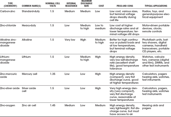
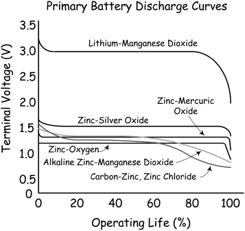
FIGURE 3.28
3.2.4 Secondary Batteries
Secondary batteries, unlike primary batteries, are rechargeable by nature. The actual discharge characteristics for secondary batteries are similar to those of primary batteries, but in terms of design, secondary batteries are made for long-term, high-power-level discharges, whereas primary batteries are designed for short discharges at low power levels. Most secondary batteries come in packages similar to those of primary batteries, with the exception of, say, lead-acid batteries and special-purpose batteries. Secondary batteries are used to power such devices as laptop computers, portable power tools, electric vehicles, emergency lighting systems, and engine starting systems.
Here are some common packages for secondary batteries:
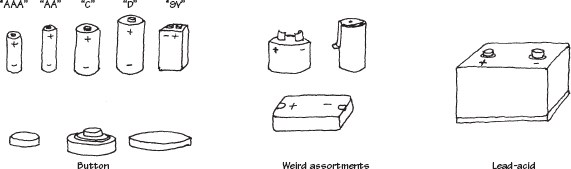
FIGURE 3.29
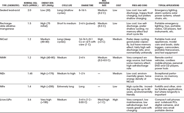
Comparing Secondary (Rechargeable) Batteries
LEAD-ACID BATTERIES
Lead-acid batteries are typically used for high-power applications, such as motorized vehicle power and battery backup applications. There are basically three types of lead-acid batteries: flooded lead-acid, valve-regulated lead-acid (VRLA), and sealed lead-acid (SLA). The flooded types must be stood upright and tend to lose electrolytes while producing gas over time. The SLA and VRLA are designed for a low overvoltage potential to prohibit the battery from reaching its gas-generating potential during discharge. However, SLA and VRLA can never be charged to their full potential. VRLA is generally used for stationary applications, while the SLA can be used in various positions. Lead-acid batteries typically come in 2-V, 4-V, 6-V, 8-V, and 12-V versions, with capacities ranging from 1 to several thousand amp-hours. The flooded lead-acid battery is used in automobiles, forklifts, wheelchairs, and UPS devices.
An SLA battery uses a gel-type electrolyte rather than a liquid to allow it to be used in any position. However, to prevent gas generation, it must be operated at a lower potential—meaning it’s never fully charged. This means that it has a relatively poor energy density—the lowest for all sealed secondary batteries. However, they’re the cheapest secondary, making them best suited for applications where low-cost, stationary power storage is the main concern. SLA batteries have the lowest self-discharge rate of any of the secondary batteries (about 5 percent per month). They do not suffer from memory effect (as displayed in NiCad batteries), and they perform well with shallow cycling; in fact, they tend to prefer it to deep cycling, although they perform well with intermittent heavy current demands, too. SLA batteries aren’t designed for fast charging—typically 8 to 16 hours for full recharge. They must also always be stored in a charged state. Leaving them in a discharged state can lead to sulfation, a condition that makes the batteries difficult, if not impossible, to recharge. Also, SLA batteries have an environmentally unfriendly electrolyte.
The basic technique for recharging lead-acid batteries, be they flooded, sealed, or valve-regulated, is to read the technical directions that come with them. If you don’t know what you’re doing—say, trying to make your own battery recharger—you may run into a serious problem, such as blowing up batteries with too much pressure, melting them, or destroying the chemistry. (The procedure for charging lead-acid batteries is different from that for NiCad and NiMH batteries in that voltage limiting is used instead of current limiting.)
NICKEL-CADMIUM (NiCAD) BATTERIES
Nickel-cadmium batteries are made using nickel hydroxide as the positive electrode and cadmium hydroxide as the negative electrode, with potassium hydroxide as the electrolyte. Nickel-cadmium batteries have been a very popular rechargeable battery over the years; however, with the introduction of NiMH batteries, they have seen a decline in use. In practical terms, NiCad batteries don’t last very long before needing a recharge. They put out less voltage (per cell) than a standard alkaline (1.2 V versus 1.5 V for alkaline). This means that applications that require four or more alkaline batteries might not work at all with comparable-sized NiCad batteries. During discharge, the average voltage of a sealed NiCad cell is about 1.2 V per cell. At nominal discharge rates, the characteristic is very nearly flat until the cell approaches full discharge. The battery provides most of its energy above 1.0 V per cell. The self-discharge rate of a NiCad is not great, either—around two to three months. However, like SLAs, sealed NiCads can be used in virtually any position. NiCads have a higher energy density than SLAs (about twice as much), and with a relatively low cost, they are popular for powering compact portable equipment: cordless power tools, model boats and cars, and appliances such as flashlights and vacuum cleaners. NiCads suffer from memory effect and are therefore not really suitable for applications that involve shallow cycling or spending most of their time on a float charger. They perform best in situations where they’re deeply cycled. They have a high number of charge/discharge cycles—around 1000.
Use a recommended charger—a constant current–type charger with due regard for heat dissipation and wattage rating. Improper charging can cause heat damage or even high-pressure rupture. Observe proper charging polarity. The safe charge rate for sealed NiCad cells for extended charge periods is 10 hours, or C/10 rate.
NICKEL METAL HYDRIDE (NiMH) BATTERIES
NiMH batteries are very popular secondary batteries, replacing NiCad batteries in many applications. NiMH batteries use a nickel/nickel hydroxide positive electrode, a hydrogen-storage alloy (such as lanthanum-nickel or zirconium-nickel) as a negative electrode, and potassium hydroxide as the electrolyte. They have a higher energy density than standard NiCad batteries (about 30 to 40 percent higher) and don’t require special disposal requirements, either. The nominal voltage of a NiMH battery is 1.2 V per cell, which must be taken into consideration when substituting them into devices that use standard 1.5-V cells such as alkaline cells. They self-discharge in about two to three months and do display some memory effect, but not as bad as NiCad batteries. They are not as happy with a deep discharge cycle as a NiCad battery, and they tend to have a shorter work life. Best results are achieved with load currents of 0.2-C to 0.5-C (one-fifth to one-half of the rated capacity). Typical applications include remote-control vehicles and power tools (although NiMH batteries are rapidly being superceded by Li-ion and LiPo batteries).
Recharging NiMH batteries is a bit complex due to significant heat generation; the charge uses a special algorithm that requires trickle charging and temperature sensing. Unlike NiCad batteries, NiMH batteries have little memory effect. The batteries require regular full discharge to prevent crystalline formation.
Li-ION BATTERIES
Lithium is the lightest of all metals and has the highest electrochemical potential, giving it the possibility of an extremely high energy density. However, the metal itself is highly reactive. While this isn’t a problem with primary cells, it poses an explosion risk with rechargeable batteries. For these to be made safe, lithium-ion technology had to be developed; the technology uses lithium ions from chemicals such as lithium-cobalt dioxide, instead of the metal itself. Typical Li-ion batteries have a negative electrode of aluminum coated with a lithium compound such as lithium-cobalt dioxide, lithium-nickel dioxide, or lithium-manganese dioxide. The positive electrode is generally of copper, coated with carbon (generally either graphite or coke), while the electrolyte is a lithium salt such as lithium-phosphorous hexafluoride, dissolved in an organic solvent such as a mixture of ethylene carbonate and dimethyl carbonate. Li-ion batteries have roughly twice the energy density of NiCads, making them the most compact rechargeable yet in terms of energy storage. Unlike NiCad or NiMH batteries, they are not subject to memory effect, and have a relatively low self-discharge rate—about 6 percent per month, less than half that of NiCads. They are also capable of moderately deep discharging, although not as deep as NiCads, as they have a higher internal resistance. On the other hand, Li-ion batteries cannot be charged as rapidly as NiCads, and they cannot be trickle or float charged, either. They also are significantly more costly than either NiCads or NiMH batteries, making them the most expensive rechargeables of all. Part of this is that they must be provided with built-in protection against both excessive discharging and overcharging (both of which pose a safety risk). Most Li-ion batteries are therefore supplied in self-contained battery packs, complete with “smart” protective circuitry. They are subject to aging, even if not used, and have moderate discharge currents. The main applications for Li-ion batteries are in places where as much energy as possible needs to be stored in the smallest possible space, and with as little weight as possible. They are found in laptop computers, PDAs, camcorders, and cell phones.
Li-ion batteries require special voltage-limiting recharging devices. Commercial Li-ion battery packs contain a protection circuit that prevents the cell voltage from going too high while charging. The typical safety threshold is set to 4.30 V/cell. In addition, temperature sensing disconnects the charging device if the internal temperature approaches 90°C (194°F). Most cells feature a mechanical pressure switch that permanently interrupts the current path if a safe pressure threshold is exceeded. The charge time of all Li-ion batteries, when charged at a 1-C initial current, is about three hours. The battery remains cool during charge. Full charge is attained after the voltage has reached the upper voltage threshold and the current has dropped and leveled off at about 3 percent of the nominal charge current. Increasing the charge current on a Li-ion charger does not shorten the charge time by much. Although the voltage peak is reached more quickly with higher current, the topping charge will take longer.
LITHIUM POLYMER (Li-POLYMER) BATTERIES
The lithium polymer batteries are a lower-cost version of the Li-ion batteries. Their chemistry is similar to that of the Li-ion in terms of energy density, but uses a dry solid polymer electrolyte only. This electrolyte resembles a plastic-like film that does not conduct electricity but allows an exchange of ions (electrically charged atoms or groups of atoms). The dry polymer is more cost effective during fabrication, and the overall design is rugged, safe, and thin. With a cell thickness measuring as little as 1 mm, it is possible to use this battery in thin compact devices where space is an issue. It is possible to create designs which form part of a protective housing, are in the shape of a mat that can be rolled up, or are even embedded into a carrying case or piece of clothing. Such innovative batteries are still a few years away, especially for the commercial market.
Unfortunately, the dry Li-polymer suffers from poor ion conductivity, due to high internal resistance; it cannot deliver the current bursts needed for modern communication devices. However, it tends to increase in conductivity as the temperature rises, a characteristic suitable for hot climates. To make a small Li-polymer battery more conductive, some gelled electrolyte may be added. Most of the commercial Li-polymer batteries used today for mobile phones are hybrids and contain gelled electrolytes.
The charge process of a Li-polymer battery is similar to that of the Li-ion battery. The typical charge time is around one to three hours. Li-polymer batteries with gelled electrolyte, on the other hand, are almost identical to Li-ion batteries. In fact, the same charge algorithm can be applied.
NICKEL-ZINC (NiZn) BATTERIES
Nickel-zinc batteries are commonly used in light electric vehicles. They are considered the next generation of batteries used for high-drain applications, and are expected to replace sealed lead-acid batteries due to their higher energy densities (up to 70 percent lighter for the same power). They are also relatively cheap compared to NiCad batteries.
NiZn batteries are chemically very similar to NiCad batteries; both use an alkaline electrolyte and a nickel electrode, but they differ significantly in their voltage. The NiZn cell delivers more than 0.4 V of additional voltage both at open circuit and under load. With the additional 0.4 V per cell, multicell batteries can be constructed in smaller packages. For example, a 19.2-V pack can replace a 14.4-V NiCad pack, representing a 25 percent lower cell space and delivering higher power and a 45 percent lower impedance. They are also less expensive than most rechargeables. They are safe (abuse-tolerant). The life cycle is a bit better than for NiCad batteries for typical applications. They have superior shelf life when compared to lead-acid. Also, they are considered environmentally green—both nickel and zinc are nontoxic and easily recycled.
In terms of recharge times, it takes less than two hours to achieve full recharge; there is an 80 percent charge in one hour. This feature makes them useful in cordless power tools. Their high energy density and high discharge rate make them suitable for applications that demand large amounts of power in small, lightweight packages. They are found in cordless power tools, UPS systems, electric scooters, high-intensity dc lighting and the like.
NICKEL-IRON (NiFe) BATTERIES
Nickel-iron batteries, also called nickel alkaline or NiFe batteries, were introduced in 1900 by Thomas Edison. These are very robust batteries that are tolerant of abuse and can have very long life spans (30 years or more). The open-circuit voltage of these cells is 1.4 V, and the discharge voltage is about 1.2 V. They withstand overcharge and over-discharge. They accept high depth of discharge (deep cycling) and can remain discharged for long periods without damage, unlike lead-acid batteries that need to be stored in a charged state. They are, however, very heavy and bulky. Also, the low reactivity of the active components limits high-discharge performance. The cells take a charge slowly, give it up slowly, and have a steep voltage dropoff with state of charge. Furthermore, they have a low energy density compared to other secondary batteries, and a high self-discharge rate. NiFe batteries are used in applications similar to those for lead-acid batteries, but oriented toward a necessity of longevity. (A typical lead-acid battery will last around five years, compared to around 30 to 80 years for a NiFe battery.)
Rechargeable alkaline-manganese, or RAM, batteries are the rechargeable version of primary alkaline batteries. Like the primary technology, they use a manganese dioxide positive electrode and potassium hydroxide electrode, but the negative electrode is now a special porous zinc gel designed to absorb hydrogen during the charging process. The separator is also laminated to prevent it being pierced by zinc dendrites. These are often considered a poor substitute for a rechargeable, as compared to a NiCad or NiMH battery. RAM batteries have a tendency to plummet in capacity over few recharge cycles. It is feasible for a RAM battery to lose 50 percent of its capacity after only eight cycles. On the positive side, they are inexpensive and readily available. They can usually be used as a direct replacement for non-rechargeable batteries, but they usually have a lower nominal voltage, making them unsuitable for some devices, except in high-drain devices like digital cameras. They have a low self-discharge rate and can be stored on standby for up to 10 years. Also, they are environmentally friendly (no toxic metals are used) and maintenance-free; there is no need for cycling or worrying about memory effect. On the short side, they have limited current-handling capability and are limited to light-duty applications such as flashlights and other low-cost portable electronic devices that require shallow cycling. Recharging a RAM battery requires a special recharger; if you charge them in a standard charger, they may explode.
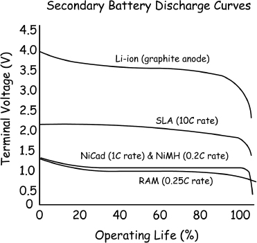
FIGURE 3.30
THE SUPERCAPACITOR
The supercapacitor isn’t really a battery but a cross between a capacitor and a battery. It resembles a regular capacitor, but uses special electrodes and some electrolytes. There are three kinds of electrode material found in a supercapacitor: high-surface-area-activated carbons, metal oxide, and conducting polymers. The one using high-surface-area-activated carbons is the most economical to manufacture. This system is also called double layer capacitor (DLC) because the energy is stored in the double layer formed near the carbon electrode surface. The electrolyte may be aqueous or organic. The aqueous electrolyte offers low internal resistance but limits the voltage to 1 V. In contrast, the organic electrolyte allows 2 and 3 V of charge, but the internal resistance is higher.
To make the supercapacitor practical for use in electronic circuits, higher voltages are needed. Connecting the cells in series accomplishes this task. If more than three or four capacitors are connected in series, voltage balancing must be used to prevent any cell from reaching overvoltage.
Supercapacitors have values from 0.22 F upwards to several F. They have higher energy storage capacity than electrolytic capacitors, but a lower capacity than a battery (approximately  that of a NiMH battery). Unlike electrochemical batteries that deliver a fairly steady voltage, the voltage of a supercapacitor drops from full voltage to zero volts without the customary flat voltage curve characteristic of most batteries. For this reason, supercapacitors are unable to deliver the full charge. The percentage of charge that is available depends on the voltage requirements of the applications. For example, a 6-V battery is allowed to discharge to 4.5 V before the equipment cuts off; the supercapacitor reaches that threshold with the first quarter of the discharge. The remaining energy slips into an unusable voltage range.
The self-discharge of the supercapacitor is substantially higher than that of the electrochemical battery. Typically, the voltage of the supercapacitor with an organic electrolyte drops from full charge to the 30 percent level in as little as 10 hours. Other supercapacitors can retain the charged energy longer. With these designs, the capacity drops from full charge to 85 percent in 10 days. In 30 days, the voltage drops to roughly 65 percent, and to 40 percent after 60 days.
The most common supercapacitor applications are memory backup and standby power for real-time clock ICs. Only in special applications can the supercapacitor be used as a direct replacement for a chemical battery. Often the supercapacitor is used in tandem with a battery (placed across its terminals, with a provision in place to limit high influx of current when equipment is turned on) to improve the current handling of the battery: during low load current the battery charges the supercapacitor; the stored energy of the supercapacitor kicks in when a high load current is requested. In this way the supercapacitor acts to filter and smooth pulsed load currents. This enhances the battery’s performance, prolongs the runtime, and even extends the longevity of the battery.
Limitations include an inability to use the full energy spectrum—depending on the application, not all energy is available. A supercapacitor has low energy density, typically holding  to the energy of an electrochemical battery. Cells have low voltages—serial connections are needed to obtain higher voltages. Voltage balancing is required if more than three capacitors are connected in series. Furthermore, the self-discharge is considerably higher than that of an electrochemical battery.
Advantages include a virtually unlimited life cycle—supercapacitors are not subject to the wear and aging experienced by electrochemical batteries. Also, low impedance can enhance pulsed current demands on a battery when placed in parallel with the battery. Supercapacitors experience rapid charging—with low-impedance versions reaching full charge within seconds. The charge method is simple—the voltage-limiting circuit compensates for self-discharge.
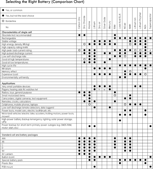
FIGURE 3.31
3.2.5 Battery Capacity
Batteries are given a capacity rating that indicates how much electrical energy they are capable of delivering over a period of time. The capacity rating is specified in terms of ampere-hours (Ah) and millampere-hours (mAh). Knowing the battery capacity, it is possible to estimate how long the battery will last before being considered dead. The following example illustrates this.
Example: A battery with a capacity of 1800 mAh is to be used in a device that draws 120 mA continuously. Ignoring possible loss in capacity as a result of load current magnitude, how long should the battery be able to deliver power?
Answer: Ideally, this would be:
Note: In reality, you must consult the battery manufacturer’s data sheets and analyze their discharge graphs (voltage as a function of time and of load current) to get an accurate determination of actual discharge time. As the load current increases, there is an apparent loss in battery capacity caused by internal resistance.
Typical capacity ratings for AAA, AA, C, D, and 9-V NiMH batteries are 1000 mAh (AAA), 2300 mAh (AA), 5000 mAh (C), 8500 mAh (D), 250 mAh (9).
C Rating
The charge and discharge currents of a battery are measured in capacity rating or C rating. The capacity represents the efficiency of a battery to store energy and its ability to transfer this energy to a load. Most portable batteries, with the exception of lead-acid, are rated at 1 C. A discharge rate of 1 C draws a current equal to the rated capacity that takes one hour (h). For example, a battery rated at 1000 mAh provides 1000 mA for 1 hour if discharged at 1 C rate. The same discharge at 0.5 C provides 500 mA for 2 hours. At 2 C, the same battery delivers 2000 mA for 30 minutes. 1 C is often referred to as a 1-hour discharge; 0.5 C would be 2 hours, and 0.1C would be a 10-hour discharge. The discrepancy in C rates between different batteries is largely dependent on the internal resistance.
Example: Determine the discharge time and average current output of a battery with a capacity rating of 1000 mAh if it is discharged at 1 C. How long would it take to discharge at 5 C, 2 C, 0.5 C, 0.2 C, and 0.05 C?
Answer: At 1 C, the battery is attached to a load drawing 1000 mA (rated capacity/hour), so the discharge time is:
t = 1 hC/C rating = 1 hC/1 C = 1 h
At 5 C, the battery is attached to a load drawing 5000 mA (five times rated capacity/hour), so the discharge time is:
t = 1 hC/C rating = 1 hC/5 C = 0.2 h
At 2 C, the battery is attached to a load drawing 2000 mA (two times rated capacity/hour), so the discharge time is:
t = 1 hC/C rating = 1 hC/2 C = 0.5 h
At 0.5 C, the battery is attached to a load drawing 500 mA (half the rated capacity/hour), so the discharge time is:
t = 1 hC/C rating = 1 hC/0.5 C = 2 h
At 0.2 C, the battery is attached to a load drawing 200 mA (20 percent rated capacity/hour) so the discharge time is:
t = 1 hC/C rating = 1 hC/0.2 C = 5 h
At 0.05 C, the battery is attached to a load drawing 50 mA (5 percent rated capacity/hour) so the discharge time is:
t = 1 hC/C rating = 1 hC/0.05 C = 20 h
Again, note that these values are estimates. When load currents increase (especially when C values get large), the capacity level drops below nominal values—due to nonideal internal characteristics such as internal resistance—and must be determined using manufacturer’s discharge curves and Peurkert’s equation. Do a search of the Internet, using “Peurkert’s equation” as a keyword, to learn more.
3.2.6 Note on Internal Voltage Drop of a Battery
Batteries have an internal resistance that is a result of the imperfect conducting elements that make up the battery (resistance in electrodes and electrolytes). Though the internal resistance may appear low (around 0.1 Ω for an AA alkaline battery, or 1 to 2 Ω for a 9-V alkaline battery), it can cause a noticeable drop in output voltage if a low-resistance (high-current) load is attached to it. Without a load, we can measure the open-circuit voltage of a battery, as shown in Fig. 3.32a. This voltage is essentially equal to the battery’s rated nominal voltage—the voltmeter has such a high input resistance that it draws practically no current, so there is no appreciable voltage drop. However, if we attach a load to the battery, as shown in Fig. 3.32, the output terminal voltage of the battery drops. By treating the internal resistance Rin and the load resistance Rload as a voltage divider, you can calculate the true output voltage present across the load—see the equation in Fig. 3.32b.
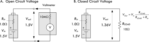
FIGURE 3.32
Batteries with large internal resistances show poor performance in supplying high current pulses. (Consult the battery comparison section and tables to determine which batteries are best suited for high-current, high-pulse applications.) Internal resistance also increases as the battery discharges. For example, a typical alkaline AA battery may start out with an internal resistance of 0.15 Ω when fresh, but may increase to 0.75 Ω when 90 percent discharged. The following list shows typical internal resistance for various batteries found in catalogs. The values listed should not be assumed to be universal—you must check the specs for your particular batteries.
| 9-V zinc carbon | 35 Ω |
| 9-V lithium | 16 to 18 Ω |
| 9-V alkaline | 1 to 2 Ω |
| AA alkaline | 0.15 Ω (0.30 Ω at 50 percent discharge) |
| AA NiMH | 0.02 Ω (0.04 Ω at 50 percent discharge) |
| D Alkaline | 0.1 Ω |
| D NiCad | 0.009 Ω |
| D SLA | 0.006 Ω |
| AC13 zinc air | 5 Ω |
| 76 silver | 10 Ω |
| 675 mercury | 10 Ω |
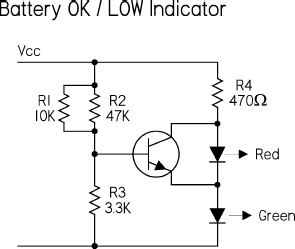
Here a green LED is used to indicate that the battery is okay. This stays on all the time to indicate that the battery is live, and the red LED comes on when the battery voltage falls below the set threshold. A green LED has around 2.0 V on when it is illuminated. This value varies a bit with different manufacturers, but is pretty well matched within any batch. Add the base emitter voltage, and you need 2.6 V on the base of the right transistor (i.e., across the 3k3) to turn on the transistor. 2.6 V across 3k3 needs 9.1 across the supply rail. Below this threshold voltage, the transistor is off and the red LED is on. Above this voltage, the red LED is off. By adjusting the values of the three resistors, you can alter the threshold level. We’ll discuss transistors and LEDs later on in this book.
FIGURE 3.33
3.3 Switches
A switch is a mechanical device that interrupts or diverts electric current flow within a circuit.
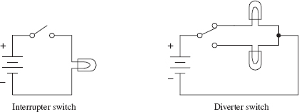
FIGURE 3.34
Two slider-type switches are shown in Fig. 3.35. The switch in Fig. 3.35a acts as an interrupter, whereas the switch in Fig. 3.35b acts as a diverter.
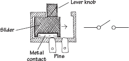
(a) When the lever is pushed to the right, the metal strip bridges the gap between the two contacts of the switch, thus allowing current to flow. When the lever is pushed to the left, the bridge is broken, and current will not flow.
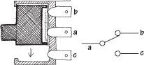
(b) When the lever is pushed upward, a conductive bridge is made between contacts a and b. When the lever is pushed downward, the conductive bridge is relocated to a position where current can flow between contact a and c.
FIGURE 3.35
Other kinds of switches, such as push-button switches, rocker switches, magnetic-reed switches, etc., work a bit differently than slider switches. For example, a magnetic-reed switch uses two thin pieces of leaflike metal contacts that can be forced together by a magnetic field. This switch, as well as a number of other unique switches, will be discussed later on in this section.
3.3.2 Describing a Switch
A switch is characterized by its number of poles and by its number of throws. A pole represents, say, contact a in Fig. 3.35b. A throw, on the other hand, represents the particular contact-to-contact connection, say, the connection between contact a and contact b or the connection between contact a and contact c in Fig. 3.35b. In terms of describing a switch, the following format is used: (number of poles) “P” and (number of throws) “T.” The letter P symbolizes “pole,” and the letter T symbolizes “throw.” When specifying the number of poles and the number of throws, a convention must be followed: When the number of poles or number of throws equals 1, the letter S, which stands for “single,” is used. When the number of poles or number of throws equals 2, the letter D, which stands for “double,” is used. When the number of poles or number of throws exceeds 2, integers such as 3, 4, or 5 are used. Here are a few examples: SPST, SPDT, DPST, DPDT, DP3T, and 3P6T. The switch shown in Fig. 3.35a represents a single-pole single-throw switch (SPST), whereas the switch in Fig. 3.35b represents a single-pole double-throw switch (SPDT).
Two important features to note about switches include whether a switch has momentary contact action and whether the switch has a center-off position. Momentary-contact switches, which include mainly pushbutton switches, are used when it is necessary to only briefly open or close a connection. Momentary-contact switches come in either normally closed (NC) or normally open (NO) forms. A normally closed pushbutton switch acts as a closed circuit (passes current) when left untouched. A normally open pushbutton switch acts as an open circuit (broken circuit) when left untouched. Center-off position switches, which are seen in diverter switches, have an additional “off” position located between the two “on” positions. It is important to note that not all switches have center-off or momentary-contact features—these features must be specified.
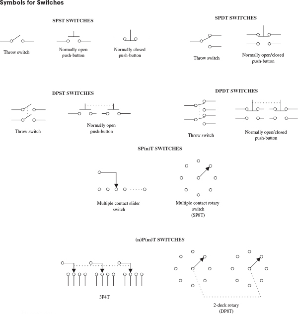
FIGURE 3.36
3.3.3 Kinds of Switches
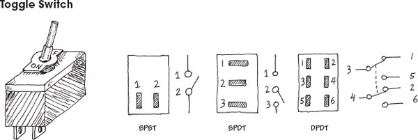
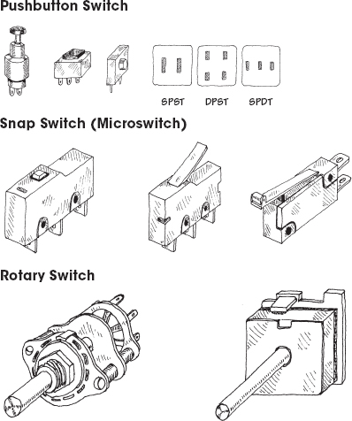
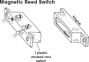
FIGURE 3.37
A reed switch consists of two closely spaced leaflike contacts that are enclosed in an air-tight container. When a magnetic field is brought nearby, the two contacts will come together (if it is a normally open reed switch) or will push apart (if it is a normally closed reed switch).
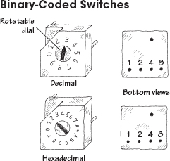
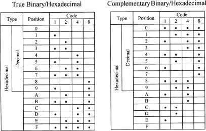
These switches are used to encode digital information. A mechanism inside the switch will “make” or “break” connections between the switch pairs according to the position of the dial on the face of the switch. These sitches come in either true binary/hexadecimal and complementary binary/hexadecimal forms. The charts below show how these switches work:
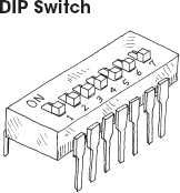
DIP stands for “dual-inline package.” The geometry of this switch’s pin-outs allows the switch to be placed in IC sockets that can be wired directly into a circuit board.
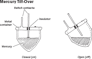
This type of switch is used as a level-sensing switch. In a normally closed mercury tilt-over switch, the switch is “on” when oriented vertically (the liquid mercury will make contact with both switch contacts). However, when the switch is tilted, the mercury will be displaced, hence breaking the conductive path.
These days, a metal ball and pair of contacts are more common than the toxic and expensive mercury.
3.3.4 Simple Switch Applications
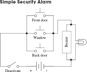
Here’s a simple home security alarm that’s triggered into action (buzzer and light go on) when one of the normally open switches is closed. Magnetic reed switches work particularly well in such applications.
FIGURE 3.38
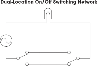
Here’s a switch network that allows an individual to turn a light on or off from either of two locations. This setup is frequently used in household wiring applications.
FIGURE 3.39
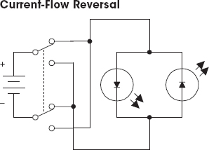
FIGURE 3.40
A DPDT switch, shown here, can be used to reverse the direction of current flow. When the switch is thrown up, current will flow throw the left light-emitting diode (LED). When the switch is thrown down, current will flow throw the right LED. (LEDs only allow current to flow in one direction.)
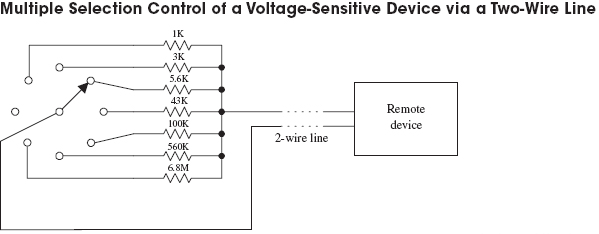
FIGURE 3.41
Say you want to control a remote device by means of a two-wire line. Let’s also assume that the remote device has seven different operational settings. One way of controlling the device would be to design the device in such a way that if an individual resistor within the device circuit were to be altered, a new function would be enacted. The resistor may be part of a voltage divider, may be attached in some way to a series of window comparators (see op amps), or may have an analog-to-digital converter interface. After figuring out what valued resistor enacts each new function, choose the appropriate valued resistors and place them together with a rotary switch. Controlling the remote device becomes a simple matter of turning the rotary switch to select the appropriate resistor.
3.4 Relays
Relays are electrically actuated switches. The three basic kinds of relays include mechanical relays, reed relays, and solid-state relays. For a typical mechanical relay, a current sent through a coil magnet acts to pull a flexible, spring-loaded conductive plate from one switch contact to another. Reed relays consist of a pair of reeds (thin, flexible metal strips) that spring together whenever a current is sent through an encapsulating wire coil. A solid-state relay is a device that can be made to switch states by applying external voltages across n-type and p-type semiconductive junctions (see Chap. 4). In general, mechanical relays are designed for high currents (typically 2 to 15 A) and relatively slow switching (typically 10 to 100 ms). Reed relays are designed for moderate currents (typically 500 mA to 1 A) and moderately fast switching (0.2 to 2 ms). Solid-state relays, on the other hand, come with a wide range of current ratings (a few microamps for low-powered packages up to 100 A for high-power packages) and have extremely fast switching speeds (typically 1 to 100 ns). Some limitations of both reed relays and solid-state relays include limited switching arrangements (type of switch section) and a tendency to become damaged by surges in power.

FIGURE 3.42
A mechanical relay’s switch section comes in many of the standard manual switch arrangements (e.g., SPST, SPDT, DPDT, etc.). Reed relays and solid-state relays, unlike mechanical relays, typically are limited to SPST switching. Some of the common symbols used to represent relays are shown below.
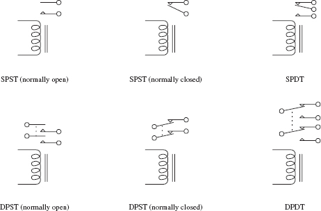
FIGURE 3.43
The voltage used to activate a given relay may be either dc or ac. For, example, when an ac current is fed through a mechanical relay with an ac coil, the flexible-metal conductive plate is pulled toward one switch contact and is held in place as long as the current is applied, regardless of the alternating current. If a dc coil is supplied by an alternating current, its metal plate will flip back and forth as the polarity of the applied current changes.
Mechanical relays also come with a latching feature that gives them a kind of memory. When one control pulse is applied to a latching relay, its switch closes. Even when the control pulse is removed, the switch remains in the closed state. To open the switch, a separate control pulse must be applied.
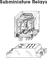
Typical mechanical relays are designed for switching relatively large currents. They come with either dc or ac coils. Dc-actuated relays typically come with excitation-voltage ratings of 6, 12, and 24 V dc, with coil resistances (coil ohms) of about 40, 160, and 650 Ω, respectively. ac-actuated relays typically come with excitation-voltage ratings of 110 and 240 V ac, with coil resistances of about 3400 and 13600 Ω, respectively. Switching speeds range from about 10 to 100 ms, and current ratings range from about 2 to 15 A.
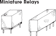
Miniature relays are similar to subminiature relays, but they are designed for greater sensitivity and lower-level currents. They are almost exclusively actuated by dc voltages but may be designed to switch ac currents. They come with excitation voltages of 5, 6, 9, and 12, and 24 V dc, with coil resistances from 50 to 3000 Ω.
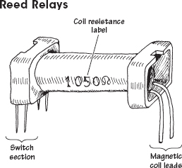
Two thin metal strips, or reeds, act as movable contacts. The reeds are placed in a glass-encapsulated container that is surrounded by a coil magnet. When current is sent through the outer coil, the reeds are forced together, thus closing the switch. The low mass of the reeds allows for quick switching, typically around 0.2 to 2 ms. These relays come with dry or sometimes mercury-wetted contacts. They are dc-actuated and are designed to switch lower-level currents, and come with excitation voltages of 5, 6, 12, and 24 V dc, with coil resistances around 250 to 2000 Ω. Leads are made for PCB mounting.
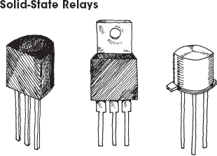
These relays are made from semiconductor materials. Solid-state relays include transistors (FETs, BJTs) and thyristors (SCRs, triacs, diacs, etc.). Solid-state relays do not have a problem with contact wear and have phenomenal switching speeds. However, these devices typically have high “on” resistances, require a bit more fine tuning, and are much less resistant to overloads when compared with electromechanical relays. Solid-state devices will be covered later in this book.
FIGURE 3.44
To make a relay change states, the voltage across the leads of its magnetic coil should be at least within ±25 percent of the relay’s specified control-voltage rating. Too much voltage may damage or destroy the magnetic coil, whereas too little voltage may not be enough to “trip” the relay or may cause the relay to act erratically (flip back and forth).
The coil of a relay acts as an inductor. Now, inductors do not like sudden changes in current. If the flow of current through a coil is suddenly interrupted, say, a switch is opened, the coil will respond by producing a sudden, very large voltage across its leads, causing a large surge of current through it. Physically speaking, this phenomenon is a result of a collapsing magnetic field within the coil as the current is terminated abruptly. [Mathematically, this can be understood by noticing how a large change in current (dI/dt) affects the voltage across a coil (V = LdI/dt).] Surges in current that result from inductive behavior can create menacing voltage spikes (as high as 1000 V) that can have some nasty effects on neighboring devices within the circuit (e.g., switches may get zapped, transistors may get zapped, individuals touching switches may get zapped, etc.). Not only are these spikes damaging to neighboring devices, they are also damaging to the relay’s switch contacts (contacts will suffer a “hard hit” from the flexible-metal conductive plate when a spike occurs in the coil).
The trick to getting rid of spikes is to use what are called transient suppressors. You can buy these devices in prepackaged form, or you can make them yourself. The following are a few simple, homemade transient suppressors that can be used with relay coils or any other kind of coil (e.g., transformer coils). Notably, the switch incorporated within the networks below is only one of a number of devices that may interrupt the current flow through a coil. In fact, a circuit may not contain a switch at all but may contain other devices (e.g., transistors, thyristors, etc.) that may have the same current-interrupting effect.
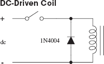
Placing a diode in reverse bias across a relay’s coil eliminates voltage spikes by going into conduction before a large voltage can form across the coil. The diode must have a peak current capability able to handle currents equivalent to the maximum current that would have been flowing through the coil before the current supply was interrupted. A good general-purpose diode that works well for just such applications is the 1N4004 diode.

When dealing with ac-actuated relays, using a diode to eliminate voltage spikes will not work—the diode will conduct on alternate half-cycles. Using two diodes in reverse parallel will not work either—the current will never make it to the coil. Instead, an RC series network placed across the coil can be used. The capacitor absorbs excessive charge, and the resistor helps control the discharge. For small loads driven from the power line, setting R = 100 Ω and C = 0.05 μF works fine for most cases. (Note: There are special devices, such as bidirectional TVs, MOVs, and MTLVs, that are designed for dc transients. See Sec. 4.5.)
FIGURE 3.45
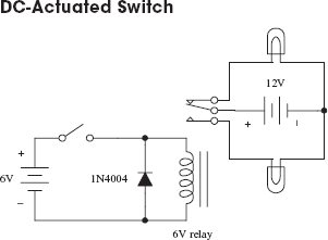
Here, a dc-powered SPDT relay is used to relay current to one of two light bulbs. When the switch in the control circuit is opened, the relay coil receives no current; hence the relay is relaxed, and current is routed to the upper bulb. When the switch in the control circuit is closed, the relay coil receives current and pulls the flexible-metal conductive plate downward, thus routing current to the lower bulb. The diode acts as a transient suppressor. Note that all components must be selected according to current and voltage ratings.
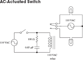
Here, an ac-actuated relay is used to switch ac current to one of two ac-rated light bulbs. The behavior in this circuit is essentially the same as in the preceding circuit. However, currents and voltages are all ac, and an RC network is used as a transient suppressor. Make sure that resistor and capacitor are rated for a potential transient current that is as large as the typical coil current. The capacitor must be rated for ac line voltage. A discrete transient suppressor (e.g., bipolar TVs or MOV) can take the place of an RC network.
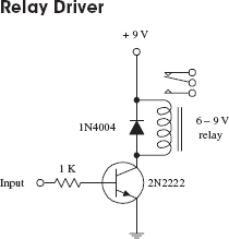
If a relay is to be driven by an arbitrary control voltage, this circuit can be used. The npn bipolar transistor acts as a current-flow control valve. With no voltage or input current applied to the transistor’s base lead, the transistor’s collector-to-emitter channel is closed, hence blocking current flow through the relay’s coil. However, if a sufficiently large voltage and input current are applied to transistor’s base lead, the transistor’s collector-to-emitter channel opens, allowing current to flow through the relay’s coil.
FIGURE 3.46
3.5 Resistors
There are various kinds of resistors available today. There are fixed resistors, variable resistors, digitally adjustable resistors, fusible resistors, photoresistors, and various resistor arrays (networks). Figure 3.47 shows schematic symbols and pictures of some of the most common types.
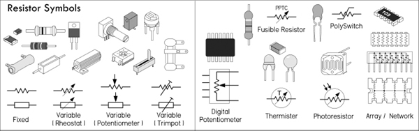
FIGURE 3.47
Resistors perform two basic functions in electronics: to limit current flow and to set voltage levels within a circuit. Figure 3.48 shows a resistor being used to reduce current flow to an LED. Without the resistor, the LED would receive excess current capable of melting its sensitive p-n junction. A variation of the LED circuit is shown with a variable resistor in series with the current-limiting resistor. The variable resistor (or potentiometer, or pot) provides additional current limiting with the desired effect of controlling the brightness of the LED.
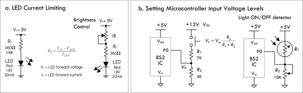
FIGURE 3.48
Figure 3.48 demonstrates how two resistors are used to create a voltage divider capable of providing a dc voltage that is a fraction of the input voltage. In this example, a voltage of 12 V is reduced to a voltage of 5 V—a usable logic HIGH level for a microcontroller’s input. A photoresistor replacing one of the voltage divider resistors acts as a variable resistor whose resistance decreases with light intensity. When this resistance decreases, the voltage present at the microcontroller’s input increases, eventually reaching a logic HIGH level. Once a logic HIGH is set up, it is then up to the microcontroller’s program to determine what course of action to take next.
The key features of current limiting and voltage setting are implemented in various ways in electronics. Resistors are used to set operating current and signal levels in circuits, provide voltage reduction, set precise gain values in precision circuits, act as shunts in ammeters and voltage meters, behave like damping agents in oscillators and timer circuits, act as bus and line terminators in digital circuits, provide feedback networks for amplifiers, and act as pullup and pulldown elements in digital circuits. They are also used in attenuators and bridge circuits. Special kinds of resistors are even used as fuses.
3.5.1 Resistance and Ohm’s Law
From Chap. 2, we learned that if a dc voltage is applied across a resistor, the amount of current that will flow through the resistor can be found using Ohm’s law—simply rearrange the equation (I = V/R). To find the power dissipated as heat by the resistor, apply the second equation below. By plugging Ohm’s law into the power equation, you also get P = I2 × R and P = V2/R, which come in handy, too.
V = I × R (Ohm’s law)
P = I × V (Power law)
R is the resistance, or the resistor, expressed in ohms (Ω), P is the power loss in watts (W), V has the voltage in volts (V), and I is the current in amperes (A).
Resistance values are given in kiloohms (kΩ) or megaohms (MΩ), where k represents 1000 and M represents 1,000,000. So a 3.3-kΩ resistor is equal to 3300 Ω, while a 2M resistor is equal to 2,000,000 Ω. Voltage, current, and power are often expressed in millivolts (mV), milliamps (mA), and milliwatts (mW), where m is equal to 0.001. 1 mV = 0.001 V; 200 mA = 0.2 A, 33 mW = 0.33 W.
As an example, in Fig. 3.49, the amount of current through a 100-Ω resistor attached to a 12-V battery is I = 12 V/100 Ω = 0.120 A or 120 mA. The power loss due to heating becomes P = 0.120 A × 12 V = 1.44 W.
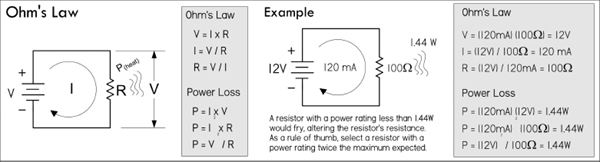
FIGURE 3.49
Determining the power loss is very important when designing circuits. All real resistors have maximum allowable power ratings that must not be exceeded. If you exceed the power rating you’ll probably end up frying your resistor, destroying the internal structure, and thus altering the resistance. Typical general-purpose resistors come in  -, ¼-, ½- and 1-W power ratings, while high-power resistors can range from 2 to several hundred watts.
So, going back to our example circuit in Fig. 3.49, the power rating of the resistor must be greater than the calculated dissipated power of 1.44 W. In reality, the power rating should be greater than this for safety. As a rule of thumb, always select a resistor that has a power rating at least twice the maximum value anticipated. Though a 2-W resistor would work in our example, a 3-W resistor would be safer. Other factors, such as ambient temperature, enclosures, resistor groupings, pulsed operation, and additional air cooling will increase or decrease the required power rating of a resistor—see the section on real resistor characteristics for more information.
3.5.2 Resistors in Series and Parallel
Rarely do you see circuits that use a single resistor alone. Usually, resistors are found connected in a variety of ways. The two fundamental ways of connecting resistors are in series and in parallel.
Resistors in Parallel
When two or more resistors are placed in parallel, the voltage across each resistor is the same, but the current through each resistor will vary with resistance. Also, the total resistance of the combination will be lower than that of the lowest resistance value present. The formula for finding the total resistance of resistors in parallel is:

The dots in the equation indicate that any number of resistors can be combined. For only two resistances in parallel (a very common case), the formula reduces to the equation below.
Example: If a 1000-Ω resistor is connected in parallel with one of 3000 Ω, what is the total resistance or equivalent resistance?
An important thing to note after applying these equations is that the current entering the top junction of the resistors in parallel equals the sum of the current entering the resistors (Iin = I1 + I2). This statement is referred to as Kirchhoff’s current law. With this law, and Ohm’s law, you come up with the current divider equation, shown to the right in Fig. 3.50. This equation comes in handy when you know the input current but not the input voltage.
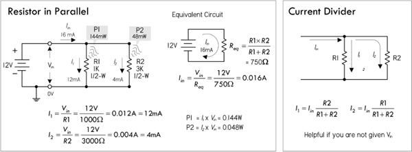
FIGURE 3.50
To find how much power resistors in parallel dissipate, apply the power law, as shown in Fig. 3.49.
Resistors in Series
When a circuit has a number of resistors connected in series, the total resistance of the circuit is the sum of the individual resistances. Also, the amount of current flowing through each resistor in series is the same, while the voltage across each resistor varies with resistance. The formula for finding the total resistance of resistors in series is:
Rtotal = R1 + R2 + R3 + R4 + … (Resistors in series)
The dots indicate that as many resistors as necessary may be added.
Example: If a 1.0-kΩ resistor is placed in series with a 2.0-kΩ resistor, what is the total resistance?
Rtotal = R1 + R2 = 1000 Ω + 2000 Ω = 3000 Ω = 3 kΩ
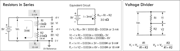
FIGURE 3.51
If we attach the two resistors to an input voltage Vin = 9 V, the total current flow, which will be the same as the individual current flow through each resistor, is:
To find the voltage drop across each resistor, apply Ohm’s law:
You can use this approach to find the voltage drop across any number of resistors in series. Also, notice that the voltage drop across each resistor is directly proportional to the resistance. The 2000-Ω resistor value is twice as large as the 2000-Ω resistor and the voltage drop across the 2000-Ω resistor is twice as large.
An important thing to notice with the voltage drops is that they all add up to the supply voltage Vin. If you start at the positive terminal of the battery (+9 V) and subtract the 3-V drop across R1 and then subtract the 6-V drop across R2, you end up with zero: +9 V − 3 V − 6 V = 0 V. Another way to put it is to say that the sum of the voltage changes around a closed path is zero. The resistors are power sinks, while the battery is a power source. It is common to assign a + sign to power sources and a − sign to power sinks. This means the voltages across the resistors have the opposite sign from the battery voltage. Adding all the voltages yields zero. This is called Kirchhoff’s voltage law.
Now, if there are only two resistors in series, you can avoid calculating currents and simply apply the following handy equations, referred to as the voltage divider equations:
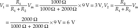
A voltmeter reading from ground to the middle of the two resistors, which we’ll call the output voltage Vout, will read 6 V, since you’re really just measuring the voltage drop across R2.
3.5.3 Reading Resistor Labels
Axial lead resistors, such as carbon composition, carbon film, and metal film, use color bands to indicate resistance values. The most common labeling scheme uses four bands: the first band represents the first digit, the second band the second digit, the third band the multiplier (as an exponent of 10), and the fourth band the tolerance (if there is no fourth band, the tolerance is 20 percent). The table in Fig. 3.52 indicates the meaning of each color in regard to number, multiplier, and tolerance.
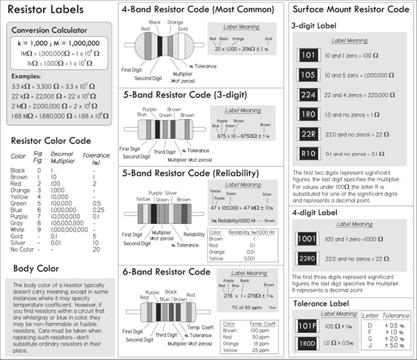
FIGURE 3.52
On precision resistors, you’ll find five bands: the first three bands are used as significant figures, the fourth band is the multiplier, while a space between the fourth and fifth band that is wider than the others is used to identify the fifth tolerance band.
Another five-band labeling scheme that is typically reserved for military-spec resistors has a fifth band reserved for reliability level. The reliability band tells you the percentage change in resistance over a time interval (e.g., 1000 hours, brown = 1 percent, red = 0.1 percent, orange = 0.01 percent, yellow = 0.001 percent).
Surface-mount resistors use either a three-digit or a four-digit label. In the three-digit scheme, the first two digits represent significant figures, and the last digit is the multiplier. For values less than 100 Ω, the letter “R” is substituted for one of the significant digits and represents a decimal point (e.g., 1R0 = 1.0 Ω).
When tolerance levels become important (e.g., narrower than around ±2 percent), an extra digit letter is placed at the end of the previous three-digit code to indicate tolerance (e.g., F = ±1). See examples in Fig. 3.52.
Precision surface-mount resistors with a four-digit code use the first three digits as significant figures, while using the last digit as the multiplier. Again, the letter “R” is used as a decimal point—see the examples in Fig. 3.52.
NOTE OF CAUTION (RESISTOR BODY COLOR)
Resistor body color usually doesn’t carry significant meaning. It sometimes represents the resistor’s temperature coefficient, but this is seldom of great importance in most hobby-type work. However, a note of caution: there are two resistor body colors that you should be aware of if you go tinkering around inside consumer electronics equipment. Resistor body colors white and blue are used to mark nonflammable resistors and fusible resistors. If you encounter this type of resistor in a circuit, do not replace it with a normal resistor. Doing so may cause a fire hazard if something goes wrong in the circuit. Nonflammable resistors and fusible resistors are designed so that they don’t catch fire when they overheat. When fusible resistors overheat, they cut the current flowing like a fuse. We’ll discuss these resistors in greater detail later in this chapter.
There are a number of things to consider when selecting a resistor for a given application. Two primary considerations include selecting the appropriate nominal resistance and power rating. The next step is to develop an acceptable tolerance for the resistor that ensures it will function properly in all extremes of the application. This task can be a bit difficult because it requires understanding a variety of nonideal characteristics that vary from one resistor family (or even between resistors in the same family) to another.
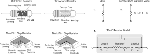
FIGURE 3.53 Some examples of real resistor construction, as well as various resistor models that are used to aid in predicting how a real resistor will behave. Model (a) represents an ideal resistor, while model (b) represents a temperature variable model for noninductive resistors. Model (c) takes into consideration the inherent inductive and capacitive elements within a resistor’s construction. For UHF and microwave designs, model (c) could be used with L representing lead inductances.
There are many different kinds of resistors out there, each with its specific set of limitations and suitable applications. A resistor that is good for one application can be disastrous in another. Resistors designated as “precision” resistors (such as precision metal film) are designed for applications where tight resistance tolerance and stability are primary considerations. They generally have restricted operating temperature limits and power dissipation ratings. “Power” resistors (such as power wirewounds) tend to be designed to optimize power dissipation at the expense of precision, and generally have extended operating temperature limits. “General-purpose” resistors (such as carbon film) tend to be somewhere in between, and are suitable for most general applications.
The following is a rundown of the important specifications used when selecting resistors. You can find detailed specifications for real resistors by checking out the manufacturers’ data sheets (e.g., www.vishay.com).
Voltage Rating
This is the maximum value of dc or RMS voltage that can be imposed across a resistor at specified ambient temperatures. The voltage rating is related to the power rating by  , where V is the voltage rating (in volts), P is the power rating (in watts), and R is the resistance (in ohms). For a given value of voltage and power rating, a critical value of resistance can be calculated. For values of resistance below the critical value, the maximum voltage is never reached; for values of resistance above the critical value, the power dissipated is lower than the rated power. One-half-watt and some 1-W resistors usually are rated only to 250 to 350 V. For high-voltage applications (e.g., a high-voltage amplifier), you may have to resort to, say, 1 W (continuous, 1000-V surge) or 2 W, 750-V-rated resistors.
Tolerance
This is expressed as the deviation (in percent) in resistance from the nominal value, measured at 25°C with no load applied. Typical resistor tolerances are 1 percent 2 percent, 5 percent, 10 percent, and 20 percent. Precision resistors, such as precision wirewounds, are made with tolerances as tight as ±0.005 percent. To understand what tolerance means, consider a 100-Ω resistor with 10 percent tolerance. The specified tolerance means that the resistor’s resistance could actually be anywhere between 90 and 110 Ω. On the other hand, a 100-Ω resistor with 1 percent tolerance has a possible resistance range from 99 to 101 Ω.
Carbon-composition resistors, as a whole, have the worst tolerance, around 5 to 20 percent. Carbon-film resistors are about 1 to 5 percent, metal-film about 1 percent, and precision metal-film resistors as low as 0.1 percent. Most wirewound resistors are from 1 to 5 percent, while precision wirewounds can achieve ±0.005 percent tolerance. Foil resistors, a relatively new technology, can achieve 0.0005 percent. For most general-purpose applications, a resistor with a 5 percent tolerance is adequate.
Power Rating
Resistors must be operated within specified temperature limits to avoid permanent damage to the materials. The temperature limit is defined in terms of the maximum power, called the power rating, and a derating curve that is provided by the resistor manufacturers (see Fig. 3.54). The power rating of a resistor is the maximum power in watts that the resistor can safely dissipate as heat, usually specified at +25°C. Beyond +25°C, the derating curve, which plots the maximum allowable power versus the ambient temperature, is used. The derating curve is usually linearly drawn from the full-rated load temperature to the maximum allowable no-load temperature. A resistor may be operated at ambient temperatures above the maximum full-load ambient temperature if operating at lower than full-rated power capacity. The maximum allowable no-load temperature is also the maximum storage temperature for the resistor.
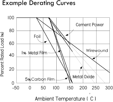
FIGURE 3.54
In regard to resistor life, any change in temperature of 30 to 40°C is tolerated—the resistor will return to its normal resistance when the temperature returns to its nominal value. However, if the resistor gets too hot to touch, you may end up permanently damaging it. For this reason, it’s important to be conservative when specifying the power rating of a resistor.
Standard power ratings for resistors include:  , , , ¼, ½, 1, 2, 5, 10, 15, 25, 50, 100, 200, 250, and 300 W. To determine the power rating for a particular application, use P = IV (P = I2R or P = V2/R), then, as a rule of thumb, select a resistor that has a power rating two to four times greater than the calculated value. Note, however, that there are many factors that go into selecting the power rating of a resistor. For more accurate design applications, you may have to weigh in other factors, such as whether resistors are grouped or enclosed within a box, whether they are fan cooled, or whether they are pulsed. In that case, you can use the chart in Fig. 3.55 to calculate an approximate power rating.
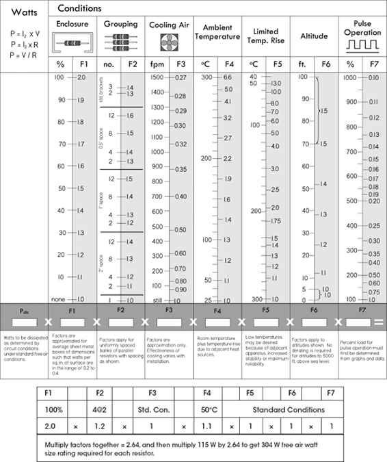
FIGURE 3.55 Calculator used for determining approximate power rating of a resistor, based on enclosure, grouping, cooling, ambient temperature, limited temperature rise, altitude, and pulsed load conditions. Example: Four resistors, each dissipating 115 W are to be mounted in a group, with spacing of two surface-to-surface, ambient to 50°C. The resistors are totally enclosed. Other factors are standard.
A kit of 1/4-, 1/2- and 1-W carbon-film and metal-film resistors is usually sufficient for most applications. A selection of 1- to 5-W wirewound resistors often comes in handy, and in rare instances you may have to resort to 10- to 600-W aluminum-housed wirewound or thick-film power resistors.
Note that in some applications (e.g., input stages to amplifiers), an effect called contact noise can be reduced by increasing the power rating (size) of the resistor—see the section on noise later in this chapter.
Temperature Coefficient of Resistance (TCR or TC)
This tells you the amount of resistance change that occurs when the temperature of a resistor changes. TC values are typically expressed as parts per million (ppm) for each degree centigrade change from some nominal temperature—usually room temperature (25°C).
So a resistor with a TC of 100 ppm will change 0.1 percent in resistance over a 10°C change, and will change 1 percent over a 100°C change (provided the temperature change is within the resistor’s rated temperature range, e.g., -55 to +145°C, measured at 25°C room temperature). A positive TC means an increase in resistance with increasing temperature, while a negative TC indicates a decreasing resistance with an increase in temperature.
Here’s another example: A 1000-Ω resistor with a TC of +200 ppm/°C is heated to 50°C. The change in resistance in parts per million is:
(200 ppm/°C) × (50°C − 27°C) = 4600 ppm
meaning the new resistance is:
1000 Ω × (1 + 4600 ppm/1,000,000 ppm) = 1004.6 Ω
There are a wide range of TC values available from ±1 ppm/°C to ± 6700 ppm/°C.
Specifying TC is important in applications where the change in resistance with temperature changes must be small. Equally important may be applications where a specific TC is required (e.g., temperature compensation circuits). Typically, there are two contributors to temperature-related resistance changes: increased temperature due to dissipated power and ambient temperature variations. The exact correspondence between dissipation, ambient temperature, and the TC is not a linear function, but rather resembles a bell-shaped or S-shaped curve. Therefore, for serious high-precision applications, you’ll have to check out the manufacturer’s resistor data sheets.
When designing circuits, you have to ask yourself which instances require high stability and low TC. For example, using a carbon-composition resistor in a stable, high-precision circuit is asking for trouble due to its high TC and weak tolerance. Using a more stable metal-film resistor with a TC of 50 to 100 ppm/°C will improve accuracy and stability considerably. Precision-film resistors have greatly improved accuracy and TCs—20, 10, 5, or 2 ppm/°C and accuracies as good as 0.01 percent. Carbon-film resistors have much higher TCs than metal-film resistors—around 500 to 800 ppm/°C. It’s easy to mistakenly insert a drifty carbon-film resistor for the intended metal-film type. Carbon-film resistors are also unique among the major resistor families, since they alone have a negative temperature coefficient. They are often used to offset the thermal effects of the other components.
As a note: often, matching TCs for pairs or sets of resistors is more important than the actual TC itself. In these cases, matched sets are available that ensure that the resistance values of the set track in the same magnitude and direction as operating temperature changes.
Frequency Response
Resistors are not perfect—they have inherent inductive and capacitive features that can alter the device’s impedance, especially as the applied ac voltage frequency increases. (Figure 3.56 shows a frequency model of a resistor.) For this reason, it’s possible for a resistor to perform like an R/C circuit, a filter, or an inductor. The primary cause of these inductive and capacitive effects results from imperfect interior layout of the resistive element as well as the resistor’s leads. In spiraled and wirewound resistors, these inductive and capacitive reactances are created by the loops and spaces formed by the spirals or turns of wire. In pulse applications, these reactive distortions result in a poor replication of the input. It is probable that a 20-ns pulse will be completely missed by a wirewound resistor, while a foil resistor, due to its superior design, achieves full replication in the time allotted. As the frequency increases, inductive reactance becomes more prevalent.
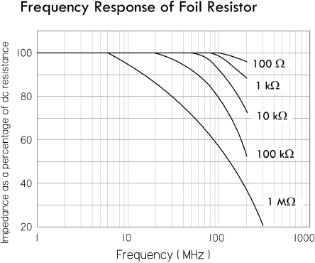
FIGURE 3.56
Even though the definition of the useful frequency range of a resistor is application dependent, typically the useful range of the resistor is the highest frequency at which the impedance differs from the resistance by more than the tolerance of the resistor. Typical reactive values for these special designs are less than 1 μH for a 500-Ω resistor, and less than 0.8-pF capacitance for a 1-MΩ resistor. A typical fast-rise-time resistor has a rise time of 20 ns or less. (Rise time is an associated parameter relating the resistor’s response to a step or pulse input.)
Wirewound resistors are notorious for their poor frequency response due to their internal coil windings. In composition resistors, frequency response also suffers from the capacitances that are formed by the many conducting particles that are held in contact by the dielectric binder. The most stable resistors for high-frequency operations are film resistors. The impedance for film resistors remains constant until around 100 MHz and then decreases at higher frequencies. In general, a resistor with a smaller diameter will have better frequency response. Most high-frequency resistors have a length-to-diameter ratio between 4:1 and 10:1. Manufacturers often supply data sheets that show the frequency response of their resistors. Impedance analyzers can also aid in modeling a resistor’s frequency response.
Noise
Resistors exhibit electrical noise in the form of small ac voltage fluctuations when dc voltage is applied. Noise is extremely difficult to measure accurately and doesn’t affect the value of the resistor but can have a devastating effect on low-level signals, digital amplifiers, high-gain amplifiers, and other applications. Noise in a resistor is a function of the applied voltage, physical dimensions, and materials. The total noise is a sum of Johnson noise, current-flow noise, noise due to cracked bodies, loose end caps, and leads. For variable resistors, noise can also be caused by the brief jumping motion of the wiper as it moves along the resistive element (e.g., wire turns).
There are three main types of resistor noise: thermal, contact, and shot noise. Thermal noise is dependent mainly on temperature, bandwidth, and resistance, while shot noise is dependent on bandwidth and average dc current. Contact noise is dependent upon average dc current, bandwidth, material geometry, and type. The following is a brief summary of the various kinds of resistor noise.
Johnson noise is temperature-dependent thermal noise. Thermal noise is also called “white noise” because the noise level is the same at all frequencies. The magnitude of thermal noise, Vrms, is dependent on the resistance value and the temperature of the resistance due to thermal agitation:
where Vrms is the root-mean-square value of the noise voltage (in volts), K is Boltzmann’s constant (1.38 × 10⁻²³ J/K), R is the resistance (in ohms), T is the temperature (in Kelvin), and Δf is the bandwidth (in hertz) over which the noise energy is measured. For resistors, the thermal noise is equivalent for equal valued resistors, regardless of material type (carbon, metal film, etc.). The only way to reduce thermal noise is to reduce the resistance value. This is why you try to avoid using a 10-MΩ resistor on the input stages of amplifiers.
Current noise varies inversely with frequency and is a function of the current flowing through the resistor and the value of the resistor—see Fig. 3.56. The magnitude of the current noise is directly proportional to the square root of the current. The current noise magnitude is usually expressed by a noise index given as the ratio of the root-mean-square current noise voltage (Vrms) over one decade bandwidth to the average voltage caused by a specified constant current passed through the resistor at a specified hot-spot temperature.
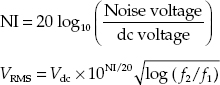
where NI is the noise index, Vdc is the dc voltage drop across the resistor, and f1 and f2 represent the frequency range over which the noise is being computed. Units of noise index are μV/V. At higher frequencies the current noise becomes less dominant compared to Johnson noise.
Contact noise is directly proportional to a constant that depends on resistor material/size and upon the average dc current. In amplifiers, for example, using a larger 2-W carbon-composition resistor will improve performance over that of a ½-W equivalent under the same conditions. The predominant noise in carbon composition, carbon film, metal oxide and metal film is composed of contact noise, which can be very large at low frequencies due to a 1/f frequency characteristic. Wirewound resistors do not have this noise—only resistors made of carbon particles. If no current (ac or dc) flows in the resistor, the noise is equal to the thermal noise. The contact noise increases as the current is increased. This means that for low-noise operation, the dc or ac current should be kept low. The material and geometry of a resistor greatly affects the contact noise, and therefore doubles the power rating of the resistor, which increases the size and area, and will reduce the contact noise generated by the resistor.
Shot noise is dependent upon current—the more average dc current through a resistor, the more noise you get. To reduce this type of noise, dc current levels must be kept low. This is often put into action in the first amplifier stage or in low-level stages such as reverb-recover amps in audio, where it is the most critical. It’s best to use a wirewound or metal-film resistor in these applications, unless you are making a high-frequency amp where inductance of the wirewound resistor comes into play.
The best resistors for low-noise applications are precision resistors. Precision wirewounds tend to be the quietest, having only thermal noise (unless terminations are faulty), but they aren’t readily available in large resistance values and are usually inductive. Precision film resistors also have extremely low noise—you’ll have to consult the manufacturers’ websites to see how noise-free modern film resistors have become. Next down the line comes metal oxide, followed by carbon film, and, last, carbon composition. Composition resistors show some degree of noise due to internal electrical contacts between conducting particles held together with the binder. And remember that, when designing critical circuits, you’ll cut down on contact noise (not applicable to wirewounds) by using the resistor with the largest practical wattage.
Don’t forget potentiometers, which are most commonly carbon composition. They generally have large values (e.g., 1 MΩ for volume control), which make them major sources of noise in an amplifier. For absolute lowest noise, conductive plastic element pots should be used, employing the lowest practical value and largest practical power rating.
Voltage Coefficient of Resistance
Resistance is not always independent of the applied voltage. The voltage coefficient of resistance is the change in resistance per unit change in voltage, expressed as a percentage of the resistance at 10 percent of rated voltage. The voltage coefficient is given by the relationship:
where R1 is the resistance at the rated voltage V1 and R2 is the resistance at 10 percent of rated voltage V2. Voltage coefficient is associated with carbon-composition and carbon-film resistors, and is a function of the resistor’s value and its composition.
Stability
This is defined as the repeatability of resistance of a resistor when measured at a reference temperature and subjected to a variety of operating and environmental conditions over time. Stability is difficult to specify and measure, since it is application dependent. Generally, wirewound and bulk-metal resistor designs are best, while designs using composition resistors are least stable. For highest resistance stability, it’s best to operate critical resistors with limited temperature rise and limited load level. Changes in temperature alternately apply and relieve stresses on the resistive element, thus causing change in resistance. The wider these temperature variations and the more rapid these changes are, the greater the change in resistance. If severe enough, this can literally destroy a resistor. Humidity can also alter the resistance by causing the insulation of the resistor to swell, thus applying pressure to the resistive element.
Reliability
This is the degree of probability that a resistor will perform its desired function. It is typically rated as mean time between failures (MTBF) or failure rate per 1,000 hours of operation. Reliability isn’t usually a critical specification for most general-purpose applications. It often does pop up in critical applications, such as those used by the military.
Temperature Rating
This is the maximum allowable temperature at which the resistor may be used. Often, two temperatures are used—one for full loads up to, say, +85°C derated to no load at +145°C. Temperature range may be specified, for example, from −55°C to +275°C.
There are numerous resistor technologies out there, with new technologies springing up all the time. The major technologies include carbon film, metal film, thick film, thin film, carbon composition, wirewound, and metal oxide. When selecting resistors for an application, you generally specify whether the resistor is to be a precision resistor, semiprecision resistor, general-purpose resistor, or power resistor.
Precision resistors have low voltage and power coefficients and excellent temperature and time stabilities, along with low noise and very low reactance. These resistors are available in metal-film or wire constructions and are typically designed for circuits having very close resistance tolerances on values.
Semiprecision resistors are smaller than precision resistors and are used primarily for current-limiting or voltage-dropping functions. They have long-term temperature stability.
General-purpose resistors are used in circuits that do not require tight resistance tolerances or long-term stability. For general-purpose resistors, initial resistance variations may be in the neighborhood of 5 percent, and the variation in resistance under full-rated power may approach 20 percent. Typically, general-purpose resistors have a high coefficient of resistance and high noise levels. However, good-quality metal film resistors are low cost and often used as general-purpose resistors.
Power resistors are used for power supplies, control circuits, and voltage dividers where operational stability of 5 percent is acceptable. Power resistors are available in wirewound and film construction. Film-type power resistors have the advantage of stability at high frequencies and have higher resistance values than wirewound resistors for a given size.
The following provides finer details highlighting the differences between the various available resistors.
Precision Wirewound
Precision wirewound resistors are very stable resistors manufactured with high tolerances. They are made by winding wire of nickel-chromium alloy onto a ceramic tube covered with a vitreous coating. They are designed to have a very low temperature coefficient of resistance (as low as 3 ppm/°C) and can achieve accuracies up to 0.005 percent. They are usually expected to operate in a temperature range from -55 to 200°C, with a maximum operating temperature of 145°C. Life is generally rated at 10,000 hours at rated temperature and load, though this can increase if operated below rated temperature. The allowable change in resistance under these conditions is about 0.10 percent. In terms of noise, there is little—only contact noise. The power-handling capability is generally low, but high-power versions are available with heat sinks.
Because of the wire-winding nature, these resistors have a component of inductances as well as capacitance associated with them. They tend to be inductive at lower frequencies and somewhat capacitive at higher frequencies, regardless of resistance value. They also have a resonant frequency—with a very low Q value. For this reason, they are unsuitable for operation above 50 kHz—forget about RF applications. Precision wirewounds are not to be used for general-purpose work, but are reserved for high-accuracy dc applications such as high-precision dc measuring equipment and as reference resistors for voltage regulators and decoding networks. (Note: There are certain precision wirewounds listed in manufacturers’ catalogs as “type HS” wirewounds. These resistors have a special winding pattern that can greatly cut down on the inductance of the winds. There are two different types of HS wirewounds: one type has almost zero inductance but greatly increased interwinding capacitance; the other type has low inductance and low capacitance and is well suited for fast-settling amplifiers.)
Once considered the best and most stable resistors, precision wirewounds now have a competitor—precision film resistors, which can match them in most every regard.
Power Wirewound 
Power wirewound resistors are similar to their precision counterparts but are designed to handle a lot more power. They will handle more power per unit volume than any other resistor. Some of the most powerful are wound similar to heater elements and require some form of cooling (e.g., fans or immersion in liquids such as mineral oil or high-density silicone liquids). These resistors are wound on a winding form, such as a ceramic tube, rod, heavily anodized aluminum, or fiberglass mandrel. The cores on which the windings are made have high heat conductivity (Steatite, Alumina, beryllium oxide, etc.). They come in various shapes—oval, flat, cylindrical—most shapes designed for heat dissipation. Chassis-mount wirewounds are generally cylindrical power resistors wound on a ceramic core molded and pressed into an aluminum heat sink and usually with heat-radiating fins. These are designed to be mounted to metal plates or a chassis to further conduct heat, which results in a rating about five times the normal power rating. Power wirewounds come in a variety of different accuracy and TCR ratings.
Metal Film 
In applications that involve fast rise times (microseconds) or high frequencies (megahertz), metal-film resistors are usually the best. They are also quite cheap and come in small sizes (e.g., surface-mount). Metal-film resistors are often considered the best compromise of all resistors. Once considered less accurate and stable than wirewounds, the technology has greatly improved, with special precision metal-film resistors reaching TC values as low as 20, 10, 5, and even 2 ppm/°C, with accuracies as good as 0.01 percent. They also have much less inductance than wirewounds and are smaller in size and less expensive. When compared to carbon-film resistors, they have lower TCs, lower noise, linearity, and better frequency characteristics and accuracy. They also surpass carbon-film resistors in terms of high-frequency characteristics. Carbon-film resistors do, however, come with higher maximum resistance values.
A metal-film resistor is made from a base metal that is vaporized in a vacuum and deposited on a ceramic rod or wafer. The resistance value is then controlled by careful adjustment of the width, length, and depth of the film. The process is very exacting, resulting in resistors with very tight tolerance values. Metal-film resistors are used extensively in surface-mount technology.
Carbon Film 
Carbon-film resistors are the most common resistor around. They are made by coating (dipping, rolling, printing, or spraying) a ceramic substrate with a special carbon-film mixture. The thickness and percentage of the carbon mixture roughly determine the resistance. To tailor resistances to precise values the ceramic pieces can be cut to a specific length. Further refinement is accomplished by cutting a spiral trimming groove—see Fig. 3.53. An alternative method of producing carbon film is to mechanically apply carbon dust dispersed in a curable polymeric binder. The material is painted on the substrate in a spiral pattern and cured at a moderately elevated temperature.
Carbon-film resistors, with 1 percent tolerances, are normally manufactured with spiral cuts and have the same kind of voltage-overload limitations as metal-film types. Though these resistors are very popular, they are drifty (TC values around 500 to 800 ppm/°C) and should not be used in circuits where metal-film resistors are intended. In other words, don’t confuse the two when building or replacing blown components. Carbon-film resistors have many of the same characteristics as carbon-composition resistors—such as being noisy and having a voltage coefficient; they outperform carbon-composition resistors in terms of lower TCR ratings and tighter tolerances. Resistor types include general-purpose, through-hole, and surface-mount devices. They also come in specialty types, such as high-power, high-voltage, and fusible. Tolerances of 1 percent or even better can be achieved; however, caution must be used in getting tight tolerances for this type of resistor because the TC, voltage coefficient, and stability may mean that it is good only for that tolerance at the time it was installed. The TC of carbon-film resistors is in the neighborhood of 100 to 200 ppm and is generally negative. Frequency response of carbon-film resistors is among the best—far better than wirewounds, and much better than carbon composition.
Carbon Composition 
Carbon-composition resistors, though not as popular as they once were, still find use in noncritical applications. They are composed of carbon particles mixed with a binder. The resistance value is varied by controlling the carbon concentration. This mixture is molded into a cylindrical shape and hardened by baking. Leads are attached axially to each end, and the assembly is encapsulated in a protective coating. Composition resistors are economical and exhibit low noise levels for resistances of about 1 MΩ. Composition resistors are usually rated for temperatures in the neighborhood of 70°C for power ranging from to 2 W. They have end-to-end shunted capacitance that may be noticed at frequencies in the neighborhood of 100 kHz, especially for resistance values above 0.3 MΩ.
However, due to poor tolerances—from 5 to 20 percent—carbon-composition resistors should not be used in critical applications. Due to their construction, they generate considerable noise that varies depending on resistance value and the package size (though above 1 MΩ they exhibit low noise).
Though composition resistors have many poor characteristics, they do quite well in overvoltage conditions. Where a metal-film resistor’s spiral gap would be zapped (breakdown causing it to short and destroy itself) during a severe overvoltage condition, a carbon-composition resistor wouldn’t be so wimpy. A carbon-composition resistor uses a large chunk of resistive material that can handle large overloads for a short time without any flashover effects (shorting). So if you’re planning to discharge a high-voltage capacitor through a series resistor where tolerances and such aren’t important, carbon composition isn’t a bad choice. Power-handling capability in relation to physical size is greater than with precision wirewounds but less than with power wirewounds.
Bulk-Metal Foil Resistors 
Foil resistors are similar in characteristics to metal films; they have better stability and lower TCRs (approaching those of precision wirewounds), and accuracy about that of metal-film resistors. High-precision versions can achieve tolerances as low as 0.005 percent and TCR values of 0.2 ppm/°C. Their main shining point is their excellent frequency response. Foil resistors are manufactured by rolling the same wire materials as used in precision wirewound resistors to make thin strips of foil. This foil is then bonded to a ceramic substrate and etched to produce the value required. Their main disadvantage is limited high-value resistance values—less than those of metal films.
Filament Resistors
The filament resistors are similar to what’s called “bathtub boat resistors,” except they are not packaged in a ceramic shell (boat). The individual resistive element with the leads already crimped is coated with an insulating material, generally a high-temperature varnish. These are used in applications where tolerance, TCR, and stability are not important but the cost is. The cost of this type is slightly higher than for carbon composition and the electrical characteristics are better.
Thin- and Thick-Film Resistors 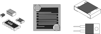
Thin-film resistors are made by depositing an extremely thin layer of NiCr resistive film (less than 1 μm) on an aluminum oxide substrate, while using NiCu materials as conducting electrodes. Thin-film technology offers extreme precision and stability (tight tolerances and low TCR values). However, these resistors have relatively limited surge capabilities due to the low mass of the resistive material. Thin-film resistors are designed as small surface-mount devices used in PCB designs and are frequently used as microwave passive and active power components such as microwave power resistors, microwave power terminations, microwave resistive power dividers, and microwave attenuators.
Thick-film resistors, in contrast to thin-film resistors, use a thicker film of RuO2, and have PdAg electrodes. These materials are also mixed with glass-based material to form a paste for printing on the substrate. The thickness of the printing material is usually 12 μm. Thick-film resistors also exhibit decent precision and stability, perhaps approaching those of thin-film resistors; however, they far exceed thin films in terms of maximum surge capacity—one to two orders of magnitude difference. Thick-film resistors come in two-lead packages and in surface-mount form. Some thick-film resistors are designed as power resistors.
Both thin-film and thick-film technologies are constantly improving, and it is difficult to specify all characteristics. Your best bet is to consult manufacturers’ data sheets for more details.
Power-Film Resistors
Power-film resistors are similar in manufacture to their respective metal-film or carbon-film resistors. They are manufactured and rated as power resistors, with power rating being the most important characteristic. Power-film resistors are available in higher maximum values than power wirewound resistors and have a very good frequency response. They are generally used in applications requiring good frequency response and/or higher maximum values. Generally, they are used for power applications, where tolerances are wider, and the temperature ratings are changed so that under full load the resistor will not exceed the maximum design temperature. Also, the physical size of the resistor is larger, and in some cases the core is made from a heat-conductive material attached to a heat sink to dissipate heat more efficiently.
Metal Oxide (Power-Metal-Oxide Film, Flameproof) 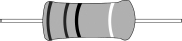
Metal-oxide resistors contain a resistance element formed by the oxidation reaction of a vapor or spray of tin-chloride solution on the heated surface of a glass or ceramic rod. The resulting tin-oxide film is adjusted to value by cutting a helix path through the film. These resistors can sustain high temperatures and electrical overloads, and have moderate-to-precision characteristics. Resistor types in this class include high-power and flameproof axial through-hole and surface-mount types. Axial versions are either blue in color or white. The outer shell of these resistors, which is flameproof like the interior, is also resistant to external heat and humidity. Metal-oxide resistors can be used to replace carbon-composition components in some applications. They are ideal for pulse-power applications. Small-sized power-type metal-oxide resistors come in a 0.5- to 5-W range, with standard tolerances of ±1 to ±5 percent and TCRs around ±300 ppm/°C. Metal-oxide resistors are used in general-purpose voltage dividers, RC timing circuits, and as pullup and pulldown resistor surge applications (e.g., RC snubber circuits, current-limiting circuits, and overload ground lines). They also come with maximum resistance values exceeding those of wirewound resistors. In general, they have decent electrical and mechanical stability and high reliability.
Fuse Resistors (Carbon Composition, Power Oxide, Metal Film) 
A fuse resistor acts as both a resistor and a fuse. Fuse resistors are designed to open-circuit (fuse) when subjected to a large surge current or fault condition. They are specially spiraled to provide the fusible function with flame-retardant coating. The fusing current is calculated based on the amount of energy required to melt the resistive material (the melt temperature plus the amount of energy required to vaporize the resistive material). These resistors will typically run hotter than a normal precision or power resistor, so that a momentary surge will bring the resistive element up to fusing temperature. Some designs create a hot spot inside the resistor to assist in this fusing. The major unknown when using fuse resistors is the heat transfer of the materials, which can be quite significant for pulses of long duration and is very difficult to calculate. Mounting fuse resistors is critical, since this will affect the fusing current. Many fuse resistors are made to mount in fuse clips for more accurate fusing characteristics. They come in a variety of types, including carbon film, metal film, thin film, and wirewound fusible. Fuse resistors are widely used in constant voltage and overload protection circuits found in battery charges, TV sets, cordless phones, PC/CPU coolers, and so on. Like traditional fuses, they come in fast- and slow-burn types.
Chip Resistor Arrays
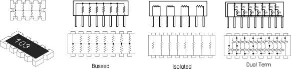
Resistor arrays contain any combination of two or more resistive elements produced on a single substrate. The resistive elements can be constructed using thick-film or thin-film technologies. These arrays come in SIP and DIP packages as well as leadless surface-mountable packages with solderable terminations. Various circuit schematics are available, including isolated resistors, single common and dual common bused resistors. Resistor arrays are used for a wide range of applications where economy of space and weight and placement costs are at a premium. Tolerances are 1 percent and 5 percent, temperature coefficients range from 50 ppm to 200 ppm, and power capabilities compare to individual resistors of similar size.
Cement Resistors 
These resistors are designed as power resistors with the added provision of being heat and flame resistant. Typical power ratings range from 1 W to 20 W or more. Tolerances are around 5 percent, with TCR ratings of around 300 ppm/°C.
Zero-Ohm Resistors (Zero-Ohm Jumpers) 
These are really nothing more than a piece of wire used for crossovers, permanent jumpers, or program jumpers (manual switch circuitry) in PCB design. They look like a signal diode with a single black stripe in the center—not to be confused with a diode that has its stripe nearer to one end. The single black stripe is meant to signify a 0-Ω value. Advantages to using these zero-ohm resistors over simple wires include ease of handling for mechanized PCB placement machinery, very low jumper-to-jumper capacitance (suitable for high-speed data lines), small footprint, and overall improvement of PC board performance.
Variable resistors are often called potentiometers, or “pots” for short, because one very common use for them is as an adjustable voltage divider. For many years they were called “volume controls,” because another very common use was for adjusting the audio volume produced by amplifiers and radio and TV receivers. Another early name for essentially the same component (when it was used simply as a variable resistance) was “rheostat,” meaning a device to set the flow (of current). See Fig. 3.57.
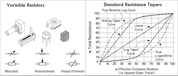
FIGURE 3.57
Pots are made in a variety of physical forms, with different kinds of resistance elements. Some pots are designed to handle frequent manual adjustment via a control knob, while others are designed to be adjusted only occasionally with a screwdriver (or similar tool) for fine-tuning a circuit. The latter type is usually referred to as a preset pot, or simply a trimpot. Most rotary pots made for manual control offer a total rotation of about 270°—¾ of a single turn. Such a limited range, however, can make accurate settings difficult, so multirevolution pots are also available. These pots have a resistance element arranged in a spiral or helix, and the wiper moves along as the control spindle is turned through multiple revolutions (typically, 10 or 20). It is possible to really home in on a resistance value with one of these pots. Multirevolution pots are rather expensive when compared to single-turn pots. For applications that require a logarithmic response (such as audio applications), you can get a pot with a logarithmic taper, as opposed to a linear taper. (Actually most logarithmic pots don’t have a true logarithmic response, as shown in Fig. 3.57. It is difficult to design such a device cheaply; making one with a near-logarithmic response isn’t so expensive.) Reverse logarithmic and antilog pots are also available—these are explained in the next section, on pot characteristics.
Trimpots can be made in circular, multiturn circular, linear-slider, and multiturn linear-slider form. Low-cost varieties generally use an open construction where the resistance element and slider are fully exposed and therefore are prone to contamination by dust and moisture. Higher-quality trimpots are generally housed inside a small plastic case, which is often hermetically sealed. Some multirevolution trimpots use a worm drive system with a circular element, while others use a linear element with a slider driven via a lead-screw. In both cases, the reduction drive is designed to have very low backlash, providing smooth and accurate adjustment.
Pots can be combined together and actuated by using a common spindle. Such pots are referred to as ganged pots. Generally, only two pots are combined this way, but it’s possible to have more. Dual ganged pots with logarithmic taper are often used in amplifier design when dealing with stereo, where you have two distinct signals.
There are various materials used in the construction of pots, such as carbon, Cermet, conductive plastic, and simple wire. Many of the characteristics that apply to fixed resistors also apply to variable resistors of the same nature—see the section on fixed resistor characteristics. Characteristics unique to pots—such as resolution, resistance taper, hop-on/hop-off resistance, and contact resistance—will differ, depending on material makeup. We will discuss these characteristics in a moment.
There are basically two ways a pot can be used in electronics. It can be used to adjust current levels or it can be used to adjust voltage levels. Figure 3.58 shows the basic setups for each scenario.
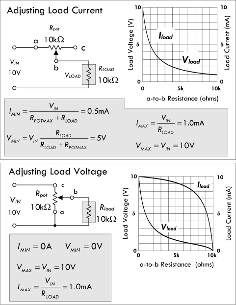
Adjusting load current: Here, a pot’s variable resistance element (a-to-b) is in series with a load. Adjusting manual control of the pot alters the current to the load. The current as a function of pot resistance is:
Notice in the graph that the load current follows a curve similar to that of the voltage. The equations in the figure display the maximum and minimum voltages and currents that can be applied across and through the load, where RPOTMAX represents the maximal pot resistance—which in this example is 10 kΩ.
Adjusting load voltage: The second configuration is essentially a variable voltage divider, which is used for adjusting the voltage applied to the load. Notice that in the graph, the load current doesn’t fall as quickly as in the previous configuration. In fact, from 0 to 5 kΩ the current falls about only 1/10 its maximum value. However, from 5 kΩ on, the drop grows significantly.
FIGURE 3.58
Resistance Taper
Pots have either linear or log tapers. Pots with linear tapers have a linear relationship between the wiper position and the resistance; for example, moving the wiper by 10 percent down the resistive element changes the resistance by 10 percent. (See Fig. 3.57.) On the other hand, a potentiometer with a log taper follows a logarithmic resistance change with wiper position, as shown in Fig. 3.57.
Naturally, the main use of common log taper pots is for controls that need to adjust a quantity in an approximate logarithmic fashion—such as for audio. Linear pots are used for most other applications. As an example, if you use a linear pot for a volume control, you’d run into problems; its adjustment grows far too rapidly as the pot is turned up from zero, while the rest of the pot’s rotation doesn’t have much control—the pot’s useful range as a volume control is squeezed into the first 60° or so of rotation, making it hard to set the right level. The log taper pot, on the other hand, is perfect as a volume control, since its logarithmic change with position matches that of the human ear’s logarithmic response to sound levels.
Now, in reality, most modern log taper pots don’t have a true logarithmic characteristic, but instead follow a rough approximation of a logarithmic curve, as shown in Fig. 3.57. The cost of manufacturing a true logarithmic taper is too high; it’s cheaper to coat a strip of material with two resistive elements of different resistive composition. This is quite acceptable as a volume control and is close to a two-slope resistance element, with the transition at about 50 percent rotation. There are indeed pots with true logarithmic response, which are made using a wirewound element on a tapered form or are made with a bulk-metal element with a carefully granulated tapered pattern.
Also shown in Fig. 3.57 are the curves for rotary reverse logarithmic and antilog taper pots, which are virtually the same as true logarithmic and log taper pots but made for the opposite, or anticlockwise, operation. These are not common nowadays, but are still available for special applications.
Resolution
This represents the smallest change in tapping ratio that can be made by moving the pot’s wiper. The resolution of wirewound pots tends to be fairly poor because the element is wound from discrete turns of resistance wire and the wiper contact can usually only slide from one turn to the next. The output of the pot, therefore, tends to vary in small regular steps, each corresponding to the voltage drop in one turn of the elements.
Pots using an etched bulk-metal element tend to have similar problems. However, pots that use a carbon-composition, hot-molded-carbon, or Cermet element tend to have somewhat better resolution because the resistance of their element is more finely graduated. Where high resolution is needed, multiturn pots tend to be more widely used than single-turn pots. It is argued that multiturn pots don’t have superior settability. The next time you need a pot with superior settability, evaluate a multiturn pot and a single-turn pot. Set each one to the desired value, tap the pots with a pencil, and tell which one stays put. Normally, it is expected that a multiturn pot, whether it has a linear or a circular layout, is better, but in reality this is not true—it can be two to four times worse than a single-turn pot because the mechanical layout of a single-turn pot is more stable and balanced.
Contact Resistance
This represents the contact resistance between the pot’s wiper and the resistance element, which has an effect on the resolution. Contact resistance also affects the noise generated by the pot, both when it’s being adjusted and when it’s simply in a fixed setting. The type of contact style and material used in pots affects contact resistance. For example, many carbon-composition pots use a simple wiper stamped from nickel-plated spring steel, with multiple fingers to give parallel wiping contacts in order to reduce contact resistance. Higher-power wirewound pots may use a wiper with a brush made from a single block of carbon, but the block is made with a loading of copper powder to keep the contact resistance as low as possible. High-grade pots with Cermet or bull-metal elements generally have a multifinger spring metal wiper of gold-plated phosphor bronze or steel. Many small trimpots of the cheaper variety have a simple spring metal wiper with a pressed dimple contact that touches the element. This is okay when the trimpot doesn’t get a lot of adjustment, but with frequent adjustment, the contact resistance tends to rise.
Hop-on and Hop-off Resistance
Most pots, whether rotary or linear-slider in design and regardless of type of resistance element, tend to have metal contact strips at the ends of the fixed element. The wiper contact generally touches and rests on these metal strips when it’s at either extreme of its travel. However, when the wiper is moved away from these extremes, it soon hops on or off the actual resistance element. Ideally, the change in resistance that occurs at the hop-on and hop-off should be zero, so that there are no sudden changes when the pot is used as a volume control, for example. However, it isn’t easy to manufacture a pot without this flaw; the best generally keep the hop-on and hop-off resistance below about 1 percent of the total value of the resistance element. This is so low that it usually can’t be detected in most audio and similar applications.
Pot Markings
As well as being marked with a character string indicating the total value of the resistance element—for example, 100 K or 1 M—the case of a pot generally also carried a code letter showing its resistance taper curve. Today most pots are marked according to the simplified taper coding system adopted by Asian component manufacturers:
A = log taper
B = linear taper
However, in older equipment you may come across pots marked according to an earlier taper coding system:
A = linear taper
C = log or audio taper
F = antilog taper
Notice the possible source of confusion!
Don’t exceed your pot’s I and V ratings. If you put a constant voltage between the wiper and one end and turn the resistance way down, you will exceed the maximum wiper current rating and soon damage or destroy the wiper contact. Note that the power rating of most variable resistors is based on the assumption that the power dissipation is uniformly distributed over the entire element. If half of the element is required to dissipate the device’s rated power, the pot may last for a short while. However, if a quarter of the element is required to dissipate the same amount of power, the pot will fail quickly. Also, some trimming pots are not rated to carry any significant dc current through the wiper. This dc current, even a milliamp, could cause electromigration, leading to an open circuit or noisy, unreliable wiper action. Carbon pots are not likely to be degraded by such a failure.
Digital Pots
Digital pots are basically analog variable resistors whose value is set by applying a digital code to their digital input leads. The actual inner circuitry is an array of digitally controlled switches that can add or subtract segments of an integrated array of single polycrystalline resistor elements. Depending on the digital code applied, a few or all the internal integrated resistors can add in series to a desired resultant resistance. Some digital pots are quite advanced, allowing you to store wiper positions in memory. Other control signals may enable the chip, increment or decrement the resistance a given amount, and so on. Digital pots can be used as three-terminal devices or as two-terminal devices. The most common is a three-terminal device, where the digital pot acts as a voltage divider. The two-terminal method is used to make the digital pot a variable current-control device—say, to step the amount of current flow through a diode. These devices are very handy in many types of analog circuits that interface with digital, such as amplifiers where the gain is determined by the digital pot’s resistance in the feedback circuit. Another example is in filter design, where the digital pot replaces the resistance used to set the cutoff frequency. It is worth purchasing a few of these devices once you start playing with microcontrollers.
3.6 Capacitors
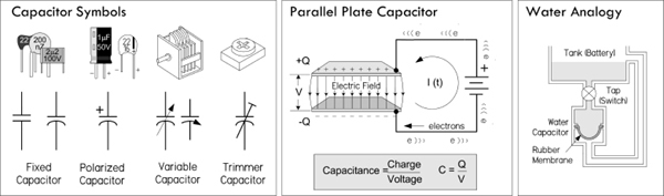
FIGURE 3.59
Capacitors perform a number of functions in electronics. One major function is simple energy storage, where charge from an applied current is stored within the capacitor and later released back into the circuit as useful current. The rate of charging and discharging can be controlled by placing a resistor in series with the capacitor. This effect is often used in high-current discharge circuits (photoflashes, actuators, etc.), as well as small energy backup supplies for low-power memory ICs. It is also used to smooth out power supply ripple, control timing in ICs, and alter the shape of waveforms.
The second major function of a capacitor when placed in series with a signal path is to block dc while allowing ac signal components to pass. A capacitor used in this way is referred to as a dc-blocking or ac-coupling capacitor. At dc, a capacitor’s impedance is ideally infinite—no current flows, no dc levels within a mixed signal are passed. However, if an ac signal is applied, the capacitor’s impedance becomes a finite value, dependent on the frequency of the signal. The higher the frequency, the lower the impedance—ideally. So, in essence, a series capacitor can be used to couple two circuits together without introducing unwanted dc shifts into the next stage, and can control how much of a given frequency signal gets through—it controls the attenuation.
Now, a capacitor placed in parallel with a signal path (i.e., to ground) has an effect opposite that of the coupling capacitor. Instead, it acts as a decoupling capacitor, allowing dc to continue along the path, while diverting high-frequency signal components to ground—the capacitor acts as a low-impedance path to ground. A similar effect, known as bypassing, is used when a capacitor is placed across a particular circuit element to divert unwanted frequencies around it. Decoupling and bypassing become fundamental when removing unwanted random high-frequency ripple and other undesired alterations within a supply voltage (or voltage-critical location) caused by random noise, or sudden current demands generated by accompanying circuit elements. Without decoupling and bypassing, many sensitive circuits, especially those incorporating digital logic ICs, have a tendency to misbehave.
Capacitors are also in passive and active filter networks, LC resonant circuits, RC snubber circuits, and so on. In these applications, it’s the reactive response to change in applied frequency that makes the capacitor useful. We’ll take a closer look at capacitor applications later in this chapter.
When a dc voltage V is applied across the leads of a capacitor, one of its “plates” charges up to a value of Q = CV, while the other plate will charge up to −Q. Here Q is the charge in coulombs (C) and C is the capacitance, or simply the proportional constant that relates Q with V. Capacitance is measured in farads, F (1 F = 1 C/1 V). Once the capacitor is charged, obtaining a voltage nearly equal to the source voltage, it will not pass any dc current—the physical separation between plates prevents this.
Capacitors come with various capacitance values, typically from 1 pF (1 × 10⁻¹²F) to 68,000 μF (0.068 F), and with various maximum voltage ratings, from a few volts to thousands of volts, depending on the type of capacitor.
In practical terms, the capacitance simply tells you how much charge can be stored within the capacitor. For example, the circuit in Fig. 3.60 shows how a 4300-μF capacitor holds more charge than a 100-μF capacitor, and, hence, will supply more current to keep the LED lit longer.
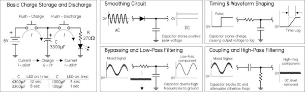
FIGURE 3.60
3.6.2 Capacitors in Parallel
When capacitors are placed in parallel, their capacitances add, just as they do for resistors in series:
Ctot = C1 + C2 + … Cn (Parallel capacitors)
Intuitively, you can think of capacitors in parallel representing one single capacitor with increased plate surface area. It’s important to note that the largest voltage that can be applied safely to a group of capacitors in parallel is limited to the voltage rating of the capacitor with the lowest voltage rating. Both the capacitance and voltage rating are usually included next to the capacitor symbol in schematics, but often the voltage rating is missing; you must figure out the rating based on the expected voltages present at that point in the circuit.
When two or more capacitors are connected in series, the total capacitance is less than that of the smallest capacitor in the group. The equivalent capacitance is calculated similarly to the resistance calculation for resistors in parallel:
Capacitors may be connected in series to enable the group to withstand a larger voltage than any individual capacitor is rated to withstand (the maximum voltage ratings add). The trade-off is a decrease in total capacitance—though that could be what you intend to do, if you can’t find a capacitor or create a parallel arrangement that gives you the desired capacitance value. Notice in Fig. 3.61 that the voltage does not divide equally among capacitors. The voltage across a single capacitor—say, C2—is a fraction of the total, expressed as (Ctot/C2)Vin. There are circuits that tap the voltage between series capacitors.
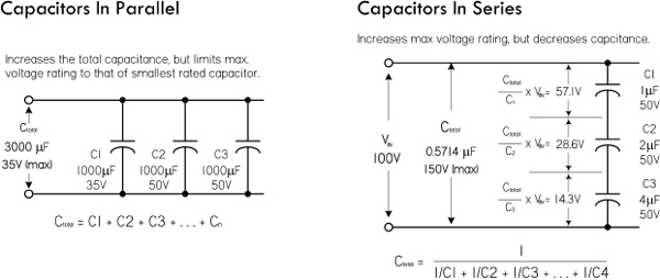
FIGURE 3.61
Use care to ensure that the voltage rating of any capacitor in the group is not exceeded. If you use capacitors in series to withstand larger voltages, it’s a good idea to also connect an equalizing resistor across each capacitor. Use resistors with about 100 Ω per volt of supply voltage, and be sure they have sufficient power-handling capability. With real capacitors, the leakage resistance of the capacitor may have more effect on the voltage division than does the capacitance. A capacitor with a high parallel resistance will have the highest voltage across it. Adding equalizing resistors reduces this effect.
3.6.4 RC Time Constant
When a capacitor is connected to a dc voltage source, it will charge up almost instantaneously. Likewise, a charged capacitor that is shorted with a wire will discharge almost instantaneously. However, with some resistance added, the rate of charge or discharge follows an exponential pattern, as shown in Fig. 3.62. There are numerous applications that use controlled charge and discharge rates, such as timing ICs, oscillators, waveform shapers, and low-discharge power backup circuits.
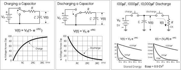
FIGURE 3.62
When charging a capacitor through a resistor, the voltage across the capacitor, with respect to time, is given as:
where V(t) is the capacitor voltage in volts at time t, VS is the source voltage, t is the time in seconds after the source voltage is applied, e = 2.718, R is the circuit resistance in ohms, and C is the capacitance in farads. Theoretically, the charging process never really finishes, but eventually the charging current drops to an unmeasurable value. A convention often used is to let t = RC, which makes V(t) = 0.632 V. The RC term is called the time constant of the circuit and is the time in seconds required to charge the capacitor to 63.2 percent of the supply voltage. The lowercase tau (τ) is often used to represent RC: τ = RC. After two time constants (t = 2RC = 2τ), the capacitor charges another 63.2 percent of the difference between the capacitor voltage at one time constant and the supply voltage, for a total change of 86.5 percent. After three time constants, the capacitor reaches 95 percent of the supply voltage, and so on, as illustrated in the graph in Fig. 3.62. After five time constants, a capacitor is considered fully charged, having reached 99.24 percent of the source voltage.
For a discharging capacitor, the following equation is used:
This expression is essentially the inverse of the previous expression for a charging capacitor. After one time constant, the capacitor voltage will have dropped by 63.2 percent from the supply voltage, so it will have reached 37.8 percent of the supply voltage. After five time constants, the capacitor is considered fully discharged; it will have dropped 99.24 percent, or down to 0.76 percent of the supply voltage.
3.6.5 Capacitive Reactance
The amount of charge that can be placed on a capacitor is proportional to the applied voltage and the capacitance (Q = CV). Within an ac circuit, the amount of charge moves back and forth in the circuit every cycle, so the rate of movement of charge (current) is proportional to voltage, capacitance, and frequency. When the effect of capacitance and frequency are considered together, they form a quantity similar to resistance. However, since no actual heat is being generated, the effect is termed capacitive reactance. The unit for reactance is the ohm, just as for resistors, and the formula for calculating the reactance of a capacitor at a particular frequency is given by:
where XC is the capacitive reactance in ohms, f is the frequency in hertz, C is the capacitance in farads, and π = 3.1416. Often, omega (ω) is used in place of 2πf.
It’s important to note that even though the unit of reactance is the ohm, there is no power dissipated in reactance. The energy stored in the capacitor during one portion of the cycle is simply returned to the circuit in the next. In other words, over a complete cycle, the average power is zero. See the graph in Fig. 3.63.
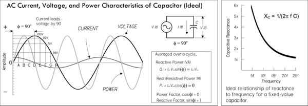
FIGURE 3.63
As an example, the reactance of a 220-pF capacitor at an applied frequency of 10 MHz is:
As you can see, the reactance decreases with an increase in frequency and/or an increase in capacitance. The right graph in Fig. 3.63 shows the reactance versus the frequency of a capacitor. Real capacitors don’t follow the graph and equation so precisely, a result of parasitic effects.
3.6.6 Real Capacitors
There are many different types of capacitors, used for various applications. Selecting the right one can be confusing. The main reason for the variety of different capacitors has to do with nonideal characteristics of real capacitors. They contain salient imperfections or parasitic effects that can mess up a particular circuit’s performance. Some capacitors, due to their construction, may have larger resistive or inductive components inherent in their design. Others may act in a nonlinear fashion or may contain dielectric memory. Understanding the effects these parasitics have in each application largely determines which capacitor you select.
The four major nonideal capacitor parameters are leakage (parallel resistance), equivalent series resistance (ESR), equivalent series inductance (ESL), and dielectric absorption (memory). Figure 3.64 shows a schematic model of a real-life capacitor. These parameters, as well as a number of other specifications are explained in the following section.
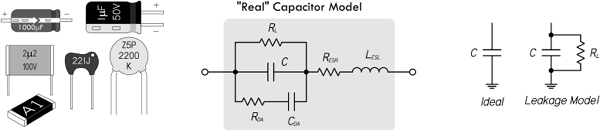
FIGURE 3.64
3.6.7 Capacitor Specifications
DC Working Voltage (DCWV)
This is the maximum safe limit of dc voltage across a capacitor to prevent dielectric breakdown—a condition that usually results in a puncture in the dielectric offering a low-resistance current path between the two plates. It is not safe to connect capacitors across an ac power line unless they are rated for it. Capacitors with dc ratings may short the line. Several manufacturers make capacitors specifically rated for use across the ac power line. For use with other ac signals, the peak value of ac voltage should not exceed the dc working voltage, unless otherwise specified in component ratings. In other words, the RMS value of ac should be 0.707 times the DCWV value or lower. With many types of capacitors, further derating is required as the operating frequency increases.
Capacitor Leakage (RL)
This is the internal leakage, as shown in the real capacitor model, that trickles off at a rate determined by the RLC time constant. Leakage becomes an important parameter when dealing with ac coupling applications and storage applications, and when capacitors are used in high-impedance circuits. Capacitors notorious for high leakage are electrolytic-type capacitors, on the order of 5 to 20 nA per μF. These capacitors are not suited for storage or high-frequency coupling applications. A better choice would be a film-type capacitor such as polypropylene or polystyrene, which has extremely low leakage current—insulation resistance typically greater than 106 MΩ.
Equivalent Series Resistance (ESR)
This is a mathematical construct, expressed in ohms, that allows all capacitor losses (resistance in capacitor leads, electrodes, dielectric losses, and leakage) at a single specific frequency to be expressed as a single series resistance with the capacitance. A high ESR causes a capacitor to dissipate more power (loss) when high-ac currents are flowing. This can degrade the capacitor. This can also have serious performance consequences at RF and in supply decoupling carrying high ripple currents. However, it is unlikely to have a significant effect in precision high-impedance, low-level analog circuitry. ESR can be calculated using the following equation:
ESR = XC/Q = XC × DF
where XC is the reactance, Q the quality factor, and DF the dissipation factor of the capacitor. Once you know the ESR, you can calculate how much power is lost due to internal heating, assuming a sine wave RMS current is known: P = IRMS2 × ESR. So a capacitor that’s considered lossy presents a large XC and is highly resistive to signal power. Using capacitors with low ESR is important in high-current, high-performance applications, such as power supplies and high-current filter networks. The lower the ESR, the higher the current-carrying ability. A few capacitors with low ESR include both mica and film types.
Equivalent Series Inductance (ESL)
The ESL of a capacitor models the inductance of the capacitor’s leads in series with the equivalent capacitance of the capacitor plates. Like ESR, ESL can also be a serious problem at high frequencies (e.g., RF), even though the precision circuitry itself may be operating at dc or low frequencies. The reason is that the transistors used in the analog circuits may have gain extending up to transition frequencies of hundreds of megahertz, or even several gigahertz, and can amplify resonances involving low values of inductance. This makes it essential that the power supply terminals of such circuits be decoupled properly at high frequency. Electrolytic, paper, or plastic-film capacitors are a poor choice for decoupling at high frequencies; they basically consist of two sheets of foil separated by sheets of plastic or paper dielectric and formed into a roll. This kind of structure has considerable self-inductance and acts more like an inductor than a capacitor at frequencies exceeding just a few megahertz. An appropriate choice for HF decoupling is a monolithic, ceramic-type capacitor, which has very low series inductance. It consists of a multilayer sandwich of metal films and ceramic dielectric, and the films are joined in parallel to bus bars rather than rolled in series. A minor trade-off is that monolithic ceramic capacitors can be microphonic (i.e., sensitive to vibration), and some types may even be self-resonant, with comparatively high Q, because of the low series resistance accompanying their low inductance. Disc ceramic capacitors are often used, but they are often quite inductive, although less expensive. Lead length of a capacitor and its construction determine the capacitor’s self-inductance and, thus, its resonant frequency.
Dissipation Factor (DF) or Tangent Delta (tanδ)
This is the ratio of all loss phenomena (dielectric and resistive) to capacitive reactance, usually expressed as a percent. It can be thought of as the ratio of energy dissipated per cycle to energy stored per cycle. It is also the ratio of the current in phase with the applied voltage to the reactive current. Dissipation factor also turns out to be equivalent to the reciprocal of the capacitor’s figure of merit, or Q, which is also often included in the manufacturer’s data sheet. DF must be given at a specific frequency to be meaningful. A lower DF indicates less power dissipated under otherwise identical conditions.
Dielectric Absorption (DA)
Monolithic ceramic capacitors are excellent for HF decoupling, but they have considerable dielectric absorption, which makes them unsuitable for use as the hold capacitor of a sample-hold amplifier. Dielectric absorption is a hysteresis-like internal charge distribution within the dielectric that causes a capacitor that is quickly discharged and then open-circuited to appear to recover some of its charge. Since the amount of charge recovered is a function of its previous charge, this is, in effect, a charge memory and will cause errors in any sample-hold amplifier where such a capacitor is used as the hold capacitor. DA is given as a percent of charge stored in a capacitor’s dielectric, as opposed to the foil surfaces. It can be approximated by the ratio of the equilibrium value “self-recharge” voltage to the voltage before discharge. Capacitors with low dielectric absorption, typically less than 0.01 percent, suitable for sample-hold applications, include polyester, polypropylene, and Teflon.
Temperature Coefficient (TC)
This represents the change in capacitance with temperature, expressed linearly as parts per million per degree centigrade (ppm/°C), or as a percent change over a specified temperature range. Most film capacitors are not linear; therefore, their TC is usually expressed as a percentage. TC should always be factored in to designs operating at temperature above or below 25°C.
Insulation Resistance (IR)
This is a measure of the resistance to a dc current flow through the capacitor under steady-state conditions. Values for film and ceramic capacitors are usually expressed in megaohm-microfarads for a given design and dielectric. The actual resistance of the capacitor is obtained by dividing the megohm-microfarads by the capacitance.
Quality Factor (Q)
This is the ratio of the energy stored to that dissipated per cycle. It is defined as Q = XC/RESR. In one respect, Q is a figure of merit that defines a circuit component’s ability to store energy compared to the energy it wastes. The rate of heat conversion is generally in proportion to the power and frequency of the applied energy. Energy entering the dielectric, however, is attenuated at a rate proportional to the frequency of the electric field and the loss tangent of the material. Thus, if a capacitor stores 1000 J of energy and dissipates only 2 J in the process, it has a Q of 500.
IRMS
This is the maximum RMS ripple current in amps at a given frequency.
Ipeak
This is the maximum peak current in amps at 25°C for nonrepetitive pulses or where the pulse time off is sufficient to allow cooling so overheating will not result.
Graphs Representing Real Capacitor Characteristics
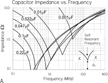
Graph A: Real capacitors aren’t entirely capacitively reactive. They also have inductive and resistive elements (ESR, ESL) that influence their overall impedance. As shown in the graph, as the frequency increases toward the capacitor’s self-resonant frequency, the impedance reaches a minimum, equal to the ESR. Past this frequency, the nonideal inductive reactance characteristic kicks in, leading to an increase in overall impedance. For many applications, the capacitor’s series-resonant frequency sets the upper frequency limit, especially where the phase angle of the capacitor is expected to maintain near 90° voltage/current relationship. The type of construction of the capacitor and lead length affect the self-inductance and thus can shift the resonant frequency. Graphs like these are given by manufacturers and are useful when selecting decoupling capacitors.
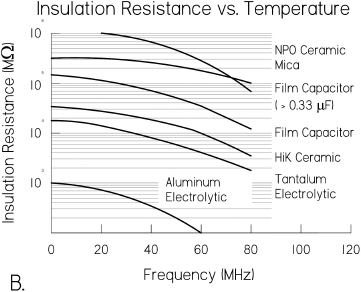
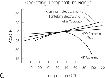
Graph C: Shows the temperature characteristics for various capacitors. Note the extraordinary curve of the HiK ceramic capacitor. Utmost attention must be used when using this type of capacitor when considering temperature-sensitive applications. NPO ceramics have the best temperature characteristic, followed by film, mica, and tantalum.
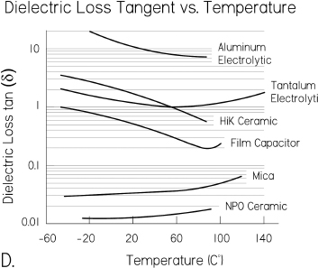
Graph D: Shows the dielectric loss tangent as a function of temperature for various capacitors.
FIGURE 3.65
3.6.8 Types of Capacitors
Here’s an overview of the various capacitors available. More in-depth coverage is provided in Table 3.7.
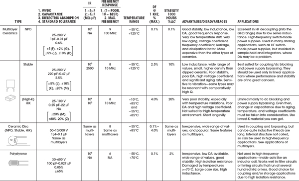
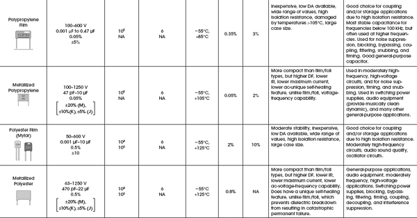
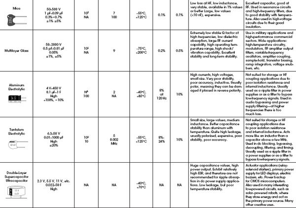
Trimmer (Variable)
These are usually designated as tuning or trimmer capacitors. Trimmer capacitors use ceramic or plastic dielectrics and are typically within the picofarad range. Trimmer capacitors often have their capacitance range printed on them but also may use the following color code: yellow (1 to 5 pF), beige (2 to 10 pF), brown (6 to 20 pF), red (10 to 40 pF), purple (10 to 60 pF), black (12 to 100 pF), and so on. They are often used for fine-tuning sensitive circuits or for compensating as a circuit ages.
Air Core (Variable)
This is an air-spaced capacitor dielectric that is the best approximation to the ideal picture. These capacitors are large when compared to those of the same value using other dielectrics. Their capacitance is very stable over a wide temperature range. Leakage losses are low, and therefore a very high Q can be obtained. To vary the capacitance, the effective surface area of an array of parallel plates is altered via a mechanical turn-knob. Tuning capacitors are used mainly in radio-tuning applications.
Vacuum
These come in both fixed and variable types. They are rated by their maximum working voltages (3 to 60 kV), capacitance (1 to 5000 pF), and currents. Losses are specified as negligible for most applications. There is excellent leakage control. These are used in high-voltage applications such as RF transmitters.
Aluminum Electrolytic
These capacitors have space between their foil plates filled with a chemical paste. When voltage is applied, a chemical reaction forms a layer of insulating material on the foil. Electrolytic capacitors are popular because they provide high capacitance values in small packages at a reasonable cost. They leak badly, have bad tolerances, drift, and have high internal inductance, limiting them to low-frequency applications. Their range is from about 0.1 to 500,000 μF. Aluminum electrolytic capacitors are very popular and are heavily used in almost every kind of circuit, since they are cheap, readily available, and good for filters and storage of large amounts of charge. They will explode, however, if the rated working voltage is exceeded or polarity is reversed. This also means you shouldn’t apply an ac voltage across an electrolytic capacitor. If an ac voltage is superimposed on a dc voltage, make sure that the peak value does not exceed the voltage rating. Aluminum electrolytic capacitors are not suited for high-frequency coupling applications due to poor isolation resistance and internal inductance. Electrolytic capacitors should not be used if the dc potential is well below the capacitor working voltage. Applications include power supply ripple filters, audio coupling, and bypassing. There are also nonpolarized electrolytic capacitors, but these are more expensive and larger than their polarized relatives.
Tantalum Electrolytic
These capacitors are made of tantalum pentoxide. Like electrolytic capacitors, they are polarized, so watch the “+” and “−.” They are smaller, lighter, and more stable; they leak less and have less inductance when compared to aluminum electrolytics, but they tend to be more expensive, have a lower maximum working voltage and capacitance, and are easily prone to damage due to current spikes. For the last reason, tantalum electrolytics are used mostly in analog signal systems that lack high current-spike noise. Tantalum capacitors are not suited for storage or high-frequency coupling applications due to poor isolation resistance and internal inductance. They should not be used if the dc potential is well below the capacitor working voltage. Applications include blocking, bypassing, decoupling, and filtering.
Polyester Film
These capacitors use a thin polyester film as their dielectric. They do not have as high a tolerance as polypropylene capacitors, but they have good temperature stability, and they are popular and cheap. Tolerances are from 5 to 10 percent. These are a good choice for coupling and/or storage applications due to high isolation resistance. They are typically used in moderately high-frequency circuits and audio and oscillator circuits.
Polypropylene Film
This type uses a polypropylene film dielectric and is used mainly when a higher tolerance is needed than what a polyester film capacitor can provide. Tolerance is about 1 percent. This is a good choice for coupling and/or storage applications due to high isolation resistance. This type exhibits stable capacitance for frequencies below 100 kHz. These capacitors are used for noise suppression, blocking, bypassing, coupling, filtering, and timing.
Silver Mica
These are made from depositing a thin layer of silver on a mica dielectric. They are very stable with respect to time (tolerances of 1 percent or less), and have a good temperature coefficient and excellent endurance, but they don’t come in high capacitance values and can be expensive. They are used in resonance circuits and high-frequency filters, due to good stability with temperature. They are also used in high-voltage circuits, because of their good insulation. Their temperature coefficient, in regard to oscillators, isn’t as low as can be achieved by other types, and some silver micas have been known to behave erratically.
Ceramic (Single-Layer)
These capacitors are constructed with materials such as titanium acid barium for the dielectric. Internally, these capacitors are not constructed as a coil, so they have low inductance and are well suited for use in higher-frequency applications. Together with electrolytics, they are the most widely used capacitor around. Ceramic capacitors come in three basic varieties:
Ultrastable or temperature compensating: This type is one of the most highly stable capacitors, made from a mixture of titanates. It has very predictable temperature coefficients (TCs) and, in general, does not have an aging characteristic. The most popular ultrastable ceramic capacitor is the NPO (negative-positive 0 ppm/°C) or COG (EIA designation); others include N030 (SIG) and N150 (P2G). The TC for these capacitors is specified in the capacitance change in parts per million (ppm) per degrees centigrade. To calculate the maximum capacitance change with temperature, the following equation is used. Here we used a 1000-pF NPO capacitor that has reached 35°C, or a change in temperature (ΔT) of 10°C above the standard reference temperature of 25°C. The TC of an NPO capacitor is 0 ± 30 ppm/°C.
Therefore, a 1000-pF capacitor subjected to a 10°C change in temperature may result in a value as high as 1000.3 pF or as low as 999.7 pF. Ultrastable capacitors are best suited for applications where stability over a wide variation of temperatures and high Q are required. Filter networks and most circuits associated with tuning and timing, as well as various types of resonant circuits, generally require ultrastable capacitors. They are particularly suitable for oscillator construction in order to compensate for frequency drift with temperature. See Table 3.7 for more details.
Semistable: These are not nearly as temperature stable as the ultrastable capacitors; however, they have a higher electrostatic capacity. All semistable capacitors vary in capacitance value under the influence of temperature, operating voltage (both ac and dc), and frequency. These capacitors are best suited for applications where high capacitance values are important, while Q stability over temperature is not a major concern. The TC for semistable capacitors is expressed as a percentage. So a 1000-pF X7R capacitor, which has a TC of ± 15 percent, might be as high as 1150 pF or as low as 850 pF at temperatures above or below 25°C. EIA TC designations are as follows: the first character defines the low-temperature limit (X = −55°C, Y = −30°C, Z = +10°C); the second character defines the high-temperature limit (5 = +85°C, 7 = +125°C); the third character defines the maximum capacitance change in percentage (V = +22, −82 percent, U = +22, −56 percent, T = +22, −33 percent, S = +22 percent, R ±15 percent, P = ±10 percent, F = ±7.5 percent, E = ±4.7 percent). See Table 3.7 and Fig. 3.66 for more details and applications.
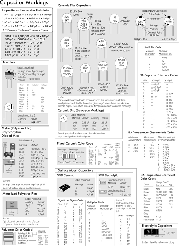
FIGURE 3.66
HiK: This variety has a high dielectric constant, or electrostatic capacity, but it has poor stability, poor DA, and a high voltage coefficient, and is sensitive to vibration—some types may be resonant, with comparatively high Q. There is very poor temperature drift, high voltage coefficient of capacitance, high voltage coefficient of dissipation, high frequency coefficient of capacitance, and significant aging rate. These also exhibit low inductance, a wide range of values, small size, and higher density than dipped ceramic. They are best suited for coupling (dc blocking) and power supply bypassing. They should be used only in linear applications where performance and stability are of no great concern.
Multilayer Ceramic
These capacitors were developed to meet the demand for high-density ceramic capacitors. They incorporate multiple printed layers of electrode plates made of thin ceramic sheets. These capacitors are more compact and have, in general, better temperature characteristics than single-layer ceramic capacitors. They are, however, more expensive. Like single-layer ceramic capacitors, they come in ultrastable, stable, and HiK types. See Table 3.7 for more details and applications.
These use a polystyrene dielectric. They are constructed like a coil inside, so they are not suitable for high-frequency applications. They are used extensively within filter circuits and timing applications, and also in coupling and storage applications due to a high isolation resistance. A warning worth noting: polystyrene capacitors exhibit a permanent change in value should they ever be exposed to temperatures much over 70°C; they do not return to their old value upon cooling.
Metallized Film (Polyester and Polypropylene)
These utilize thin conductors or plates that have a distinct size advantage over other types. They are formed by a vacuum-deposition process that laminates a film substrate with a thin aluminum coating measured in angstroms. These capacitors are used where small signal levels (low current/high impedance) and small physical size are primary factors.
Metallized-film capacitors are generally not appropriate for large-signal ac applications. Film and foil types are better suited for this purpose, since they have much thicker plates (foil) that help carry away heat buildups, thus lowering losses, extending life, and reducing effects on DF.
One major advantage of metallized-film capacitors is their self-healing characteristic—a feature resulting from the extreme thinness of the metallized electrode material. Whenever a flaw or weak spot in the dielectric results in a short condition, the stored electrons in the capacitor and the accompanying circuitry will immediately avalanche across the shorted point. This can vaporize the thin metallic electrode. The vaporized electrode forms a reasonably concentric pattern away from the point of the short. As a result of the vaporization, the short condition is removed and the capacitor is again operational. This effect is known as clearing, which is the self-healing process. In nonmetallized capacitors, the short condition results in a catastrophic permanent failure.
Some disadvantages over nonmetallized film capacitors include a slightly higher dissipation factor, slightly lower insulation resistance, lower maximum current, and lower maximum ac-voltage-frequency capability. In general, this type is a good-quality, low-drift, temperature-stable capacitor. Applications include moderately high-frequency, high-current circuits, noise suppression, timing, snubbing, switching power supplies, bypassing, and audio applications.
Supercapacitors (Double-Layer or Ultracapacitors)
These devices store extremely large amounts of charge (from 0.022 to 50 F)—much more than a typical capacitor. This level of energy storage approaches around that of a low-density battery. However, unlike a battery, the power output can be 10 times greater—a useful feature in high-current pulse applications.
Supercapacitors consist of two nonreactive porous plates suspended within an electrolyte. A voltage applied to the positive plate attracts the negative ions in the electrolyte, while the voltage on the negative plate attracts the positive ions. This effectively creates two layers of capacitive storage, one where the charges are separated at the positive plate and another where the charges are separated at the negative plate. Conductive rubber membranes contain the electrode and electrolyte material and make contact with a cell. Several cells are stacked in series to achieve the desired voltage ratings. Typical voltage ratings are 3.5 and 5.5, in keeping with their common role as backup capacitors for 3.3 V or 5 V devices.
Battery/Supercapacitor Comparison
A supercapacitor can be charged to any voltage within its voltage rating extremely quickly, and it can be stored totally discharged, while many batteries are damaged by quick charging. The state of charge of a supercapacitor is simply a function of its voltage, while the state of charge of a battery is complex and often unreliable. Though a battery will store more energy than a supercapacitor, a supercapacitor is able to deliver frequent high-power pulses without any detrimental effect, while many batteries experience reduced life under similar conditions.
Supercapacitors can be used as an intermediate power source or a bridge between batteries and conventional capacitors. Many applications benefit from the use of supercapacitors, from those requiring short power pulses to those requiring low-power, long-duration support of critical memory systems—they are capable of maintaining contents of low-dissipation CMOS memory for several months. They are excellent solutions in a number of systems when used alone or combined with other energy sources. Examples include quick-charge applications that can be charged in seconds and then discharge over a few minutes (power tools and toys), short-term support for uninterruptible power systems, where the supercapacitor provides the power for short outages, or as a bridge to a generator or other continuous backup power supply. They can provide load-leveling to an energy-rich, power-poor energy source such as a solar array.
When supercapacitors are strategically placed within battery-powered systems, they can prevent peak power–induced battery stress by supplying the peak power demands for the battery. This often allows a smaller-capacity battery to be used, and it can even extend the overall life span of the battery.
Supercapacitors exhibit high ESR, so they are not recommended for ripple absorption in dc power supply applications. See the “Capacitor Applications” section for example supercapacitor circuits.
Oil-Filled Capacitor
This type is used in high-voltage, high-current applications that generate a lot of heat—the oil cools the capacitor. Applications include induction heating, high-energy pulsing, commutation, equipment bypassing, ignitions, frequency conversion, high-voltage ripple filtering, snubbing, coupling, and spark generation. Voltages range from 1 to 300 kV, and capacitance from around 100 pF to 5000 μF. Typically, they come in large packages.
Reading Capacitor Labels
There are many different schemes used for labeling capacitors. Some use color bands, and some use combinations of numbers and letters. Capacitors may be labeled with their capacitance value, tolerance, temperature coefficient, voltage rating, or some combination of these specifications. Figure 3.66 shows several popular labeling systems.
3.6.9 Capacitor Applications
Coupling and DC Blocking
Coupling capacitors act to pass a range of ac signals from one circuit to another, while preventing any dc components from passing. This is due to the capacitor’s reactance—at dc the reactance is theoretically infinite, but at higher ac frequencies the reactance decreases. Effective coupling requires that the capacitor’s impedance be as low as possible at the frequency range of interest. If not, certain frequencies may become more attenuated than others. The formulas in Fig. 3.67 can be used to find the cutoff frequency, or −3-dB frequency (½ power point), attenuation, and phase shift, assuming ideal conditions and purely resistive load.
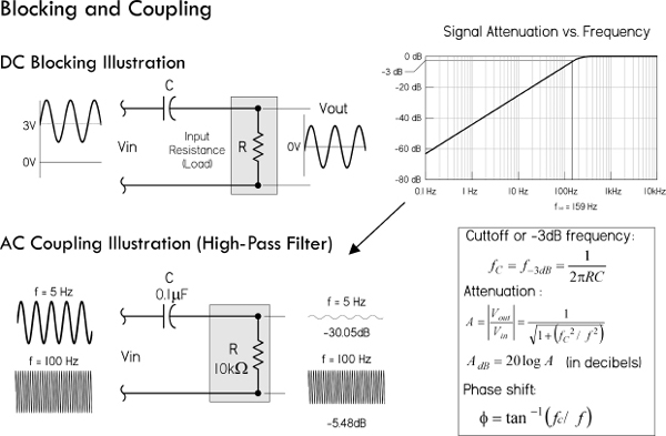
FIGURE 3.67 Blocking: A capacitor is used to block or prevent dc voltages from passing from one circuit to another. To block the dc voltage, the capacitor is placed in series with the circuit element.
Coupling: A coupling capacitor is used to couple or link together only the ac signal from one circuit element to another. The capacitor is connected in series between the input and the coupled load. Considering a purely resistive load, the attenuation and cutoff frequency (or -3-dB frequency) can be estimated by means of the formulas to the right. These formulas are based on an ideal capacitor.
Coupling: A coupling capacitor is used to couple or link together only the ac signal from one circuit element to another. The capacitor is connected in series between the input and the coupled load. Considering a purely resistive load, the attenuation and cutoff frequency (or -3-dB frequency) can be estimated by means of the formulas to the right. These formulas are based on an ideal capacitor.
Note that in many situations, the load (or coupled stage) to which the capacitor is coupled may be frequency sensitive—its impedance may change with frequency due to inductive and capacitive elements. For example, Fig. 3.70 shows how the input impedance of a transistor amplifier changes with frequency. Since the selection of the coupling capacitor determines which frequencies get attenuated, understanding the changing impedance of the coupled stage is important.
The major characteristics to look at when selecting a coupling capacitor are insulation resistance (IR), ESR, voltage rating, and overall frequency response. Consult Table 3.7 for suggested coupling capacitors. For example, for many audio applications, polypropylene and polyester film and even an electrolytic capacitor may be good choices, but for a high-frequency, high-stability decoupling application, up into the megahertz range, an NPO multilayer ceramic capacitor may be required.
Bypassing
Bypass capacitors are often used to bypass undesired alternating signals (supply ripple, noise, etc.) around a component or group of components to ground. Often the ac is removed (or greatly attenuated) from the ac/dc mixture, leaving the dc free to feed the bypassed component. Figure 3.68 shows the basics behind bypassing.
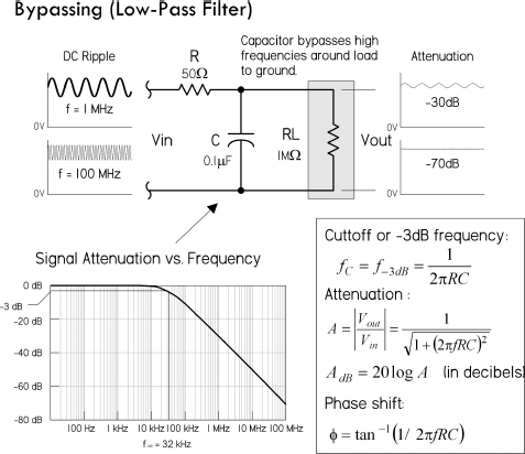
In this circuit, the RC section acts like a low-pass filter, which attenuates high frequencies from reaching the load or circuit element.
As XC < RL, signals bypass RL through C.
As XC > RL, signals pass through RL.
where XC = 1/(2πfC), the capacitor’s reactance. In other words, at high frequencies, XC gets small, so signals tend to be diverted around RL through C.
The graph in the figure shows the attenuation versus frequency response, and the equations tell you how to calculate the cutoff frequency, attenuation, and phase shift.
Note that the R in the circuit in this figure isn’t often physically present as a discrete component. It may represent, say, the inherent resistance present in the power supply line (which is usually much smaller than what’s shown). Though R helps set the frequency response, it can reduce the clamping efficiency.
FIGURE 3.68
As a general rule of thumb, the impedance of the bypass capacitor should be 10 percent of the input impedance of the circuit element.
There are many types of capacitors used for bypassing, from electrolytic to ceramic NPO. The one you choose will depend on the kind of frequency response and stability you require. Major characteristics to consider include insulation resistance (IR), ESL, and ESR. Read on.
Power Supply Decoupling (Bypassing)
Decoupling becomes very important in both digital and analog dc circuits. In these dc circuits, any slight variations in voltage within the circuit may cause improper operation. For example, in Fig. 3.69, noise (random fluctuations in supply voltage) present on the VCC line can cause problems by presenting improper voltage levels to an IC’s sensitive supply lead. (Some ICs will act erratically if this happens.) However, by placing a bypass capacitor in parallel to the IC’s input, the capacitor will bypass the high-frequency noise around the IC to ground, thus maintaining a steady dc voltage. The bypass capacitor acts to decouple the IC from the supply.
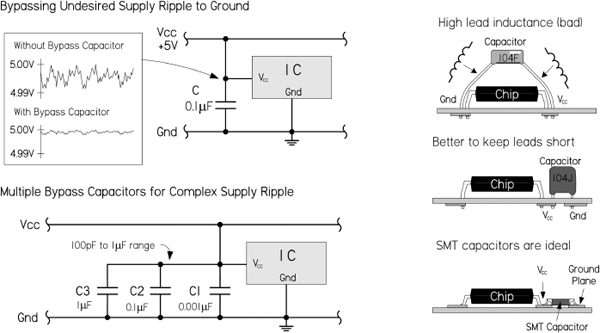
FIGURE 3.69 The top circuit uses a 0.1-μF decoupling capacitor to keep the dc supply line free of high-frequency transients. The lower circuit uses three capacitors of different capacitance levels to handle a wide range of transient frequencies.
It’s important to note that variations within the supply voltage line aren’t caused just by random low-level fluctuations. They are also caused by sudden fluctuations in voltage caused by high-current switching action that draws sudden, large amounts of current from the supply line. The more current these devices draw, the bigger the ripple in the supply line. Relay and motor switching is notorious in this regard. (Usually these devices incorporate a snubber diode or some type of local transient suppressor to limit the magnitude of the transient. However, low-level, high-frequency ringing that occurs after switching will often sneak into the line.) Even TTL and CMOS ICs can generate current spikes in the power lines, due to a transient state in which both output transistors are simultaneously on. The resistance between the 5-V supply terminals limits the supply current, and as speed increases this resistance gets smaller, and the transient currents increase to as high as 100 mA. These transient currents usually contain high frequencies due to the fast switching of the logic device. When the current spikes propagate down a power distribution system, they can develop 10- to 100-mV voltage spikes. Even worse, if an entire bus changes states, the effects are additive, resulting in transients as high as 500 mV propagating down the power lines. Such large transients wreak havoc within logic circuits.
It’s important to regard the power supply and the distribution systems (wires, PCB bus, etc.) as nonideal. The power supply contains internal resistance, and the supply distribution system (wires, PCB traces, etc.) contains small amounts of resistance, inductance, and capacitance. Any sudden demands in current from a device attached to the distribution system will thus result in a voltage dip in the supply—use Ohm’s law.
SELECTING AND PLACING DECOUPLING CAPACITORS
What Needs Bypassing: High clock-rate logic circuits and other sensitive analog circuits all require decoupling of the power supplies. As a general rule of thumb, use one 0.1-μF ceramic per digital chip, two 0.1-μF ceramics per analog chip, (one on each supply) to: (where positive and negative supplies are used) and one 1-μF tantalum per every eight ICs or per IC row, though you can often do with less. Also, a good place for bypass capacitors is on power connectors. Anytime power lines are leading off to another board or long wire, it’s a good idea to throw in a bypass capacitor; long wires act like inductive antennas, picking up electrical noise from any magnetic field. A capacitor at both ends of the wire is a good idea—a 0.01-μF or 0.001-μF capacitor connected across the line will often do the trick.
Placement: Capacitor placement is crucial for good high-frequency decoupling. Place capacitors as close as possible to the IC, between power pin and ground pin, and ensure that leads consist of wide PC tracks. Run traces from device to capacitor, then to power planes. Capacitor lead lengths must be kept short (less than 1.5 mm); even a small amount of wire has considerable inductance, which can resonate with the capacitor. Surface-mount capacitors are excellent in this regard, since you can place them almost on top of the power leads, thus eliminating lead inductance.
Size of Capacitor: The frequency of the ripple has a role in choosing the capacitor value. A rule of thumb: the higher the frequency ripple, the smaller the bypass capacitor. In Fig. 3.69, a 0.01- to 0.1-μF capacitor with a self-resonant frequency from around 10 to 100 MHz is used to handle high-frequency transients. If you have very high-frequency components in your circuit, it might be worth using a pair of capacitors in parallel—one large value (say, 0.01 μF) and one small value (say, 100 pF). If there is a complex ripple, several bypass capacitors in parallel may be used, each one targeting a slightly different frequency. For example, in the lower circuit in Fig. 3.69, C1 (1 μF) catches the lower voltage dips that are relatively low in frequency (associated with bus transients), C2 (0.1 μF) the midrange frequencies, and C3 (0.001 μF) the higher frequencies. In general, local decoupling values range from 100 pF to 1 μF. It’s generally not a good idea to place a large 1-μF capacitor on each individual IC, except in critical cases; if there is less than 10 cm of reasonably wide PC track between each IC and the capacitor, it’s possible to share it among several ICs.
Type of Capacitor: The type of capacitor used in decoupling is very important. Avoid capacitors with low ESR, high inductance, and high dissipation factor. For example, aluminum electrolytic capacitors are not a good choice for high-frequency decoupling. However, a 1-μF tantalum electrolytic, as mentioned before, is useful when decoupling at lower frequencies. Monolithic ceramic capacitors, especially surface-mount types, are an excellent choice for high-frequency decoupling due to their low ESL and good frequency response. Polyester and polypropylene capacitors are also good choices, provided you keep lead lengths short. The capacitor you eventually choose will depend on the frequency range you’re trying to eliminate. See Table 3.7 for suggested decoupling capacitors.
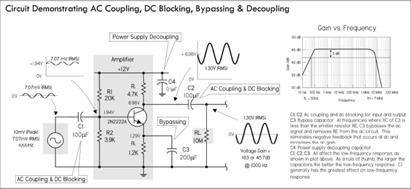
FIGURE 3.70
3.6.10 Timing and Sample and Hold
To change the voltage across a capacitor, it takes a finite amount of time—a characteristic dependent on the capacitance value and any added series resistance. The charging time, as well as the acquired voltage level, can easily be predicted, for example, by using the RC time constant. This phenomenon is put to use in timing circuits, such as oscillators, signal generators, and latch timers. An explanation of how a simple relaxation oscillator works is shown in Fig. 3.71.
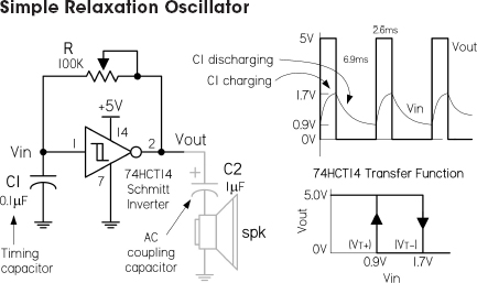
When a capacitor is charged through a resistor, its voltage follows a very predictable curve. By applying the capacitor’s voltage to a level-sensitive input of an IC, the IC will trigger an output response, once the voltage across the capacitor reaches the set trigger level. For example, in the circuit in the figure, a 74HCT14 Schmitt inverter, along with an RC network, comprise a simple squarewave oscillator. Assuming the capacitor is discharged, the inverter’s output is HIGH (+5 V). Current then passes through the resistor and starts collecting as charge within the capacitor. Once the capacitor reaches 1.7 V, the inverter interprets a HIGH input level, and sets the output LOW. C1 then begins discharging, and once its voltage reaches 0.9 V, the inverter interprets a LOW input level, and it again sets the output HIGH. The process continues. The frequency of oscillation is determined by the RC time constant. A smaller capacitance yields a higher frequency—it takes less time to charge up. Many different kinds of capacitors could be used, such as polypropylene, polyester, polystyrene (less than a few hundred kilohertz), and even electrolytic (at lower frequencies).
FIGURE 3.71
In sample-and-hold circuits, a capacitor will acquire an analog voltage level equal to that which is taken during a sample (switch closed). The stored charge within the capacitor holds onto this voltage level until a new sample is taken. See the sample-and-hold circuits in Fig. 3.72.
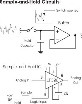
Sample-and-hold circuits are used to sample an analog signal and hold it so that it can be analyzed or converted into, say, a digital signal at one’s leisure. In the first circuit, a switch acts as a sample/hold control. Sampling begins when the switch is closed and ends when the switch is opened. When the switch is opened, the input voltage present at that exact moment will be stored in C. The op amp acts as a buffer, relaying the capacitor’s voltage to the output, but preventing the capacitor from discharging (ideally, no current enters the input of an op amp). The length of the sample voltage that can be held varies, depending on the capacitor’s leakage. Use capacitors with high ESR, low DA, low ESL, and high stability. See text.
The LF398 is a special sample-and-hold IC whose control of sample-and-hold functions is enacted by a digital input signal. An external capacitor is still needed, however, to hold the sample voltage.
FIGURE 3.72
In both timing and sample-and-hold circuits, important capacitor characteristics to look for include high insulation resistance (IR), relatively low ESR, low dielectric absorption (DA), and good capacitance stability. Polystyrene capacitors with very high IR ratings are good in many timing and storage applications, except within timing circuits that exceed a few hundred kilohertz, where ESL becomes a factor. Monolithic ceramic capacitors, though good at high frequencies, have considerably high dielectric absorption, making them unsuitable for sample-and-hold applications. Other capacitors often used in both cases include polypropylene and polyester, both of which have good IR ratings. In low-frequency relaxation-type oscillators and latch timers, electrolytic capacitors are often used, but they should not be used for sample-and-hold circuits; their leakage levels are too high to hold a constant sample voltage.
3.6.11 RC Ripple Filter
The full-wave rectifier dc supply, shown in Fig. 3.73, uses a capacitor to smooth out the rectified dc pulses in order to create a near constant dc output. The capacitor stores charge and delivers it to the load when the rectified or pulsing dc voltage decreases below its peak value. However, as it does this, the voltage drops according to the RLC time constant, until the capacitor recharges during another positive cycle. The resultant output voltage therefore takes on a small ac ripple. Since ripple is usually bad when driving sensitive circuits, it’s important to keep it as low as possible by using a large capacitance value. Figure 3.74 shows how to derive and calculate the ripple voltage, average dc voltage, and ripple factor, given the input frequency, average dc rectified voltage, capacitance, and load resistance.
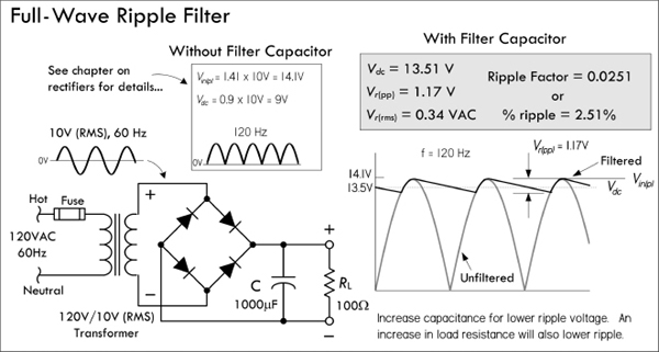
FIGURE 3.73 Here, a 1000-μF capacitor supply filter is used to reduce the output ripple voltage. With a 100-Ω load, the ripple voltage in this circuit is 0.34 VAC, or 1.17 V peak to peak. The ripple factor (rms ripple voltage divided by average dc voltage) is 0.00251. If we replaced the full-wave bridge with a half-wave rectifier, the ripple voltage would be twice as large. See equations in Fig. 3.74 and Problem 7 at the end of this chapter.
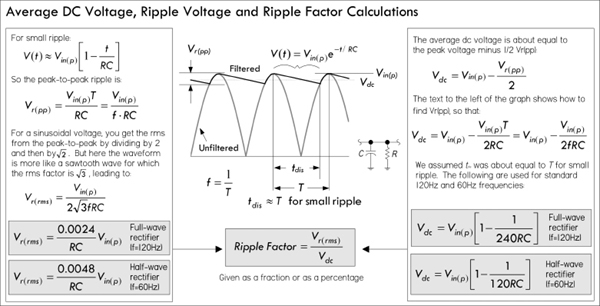
FIGURE 3.74
The ripple factor represents the maximum variation in output voltage (in rms) per the average dc output voltage. A typical and practical ripple factor to shoot for is usually around 0.05. Large capacitance values are desired to keep RF low—typically 1000 μF or more. Increasing the load resistance (decreasing load current) will also keep it down. To achieve higher capacitance levels, place filter capacitors in parallel.
Note that many times you’ll probably include a voltage regulator IC between the filter capacitor and load to combat ac-line surges and maintain a constant output voltage with changing load-current demands. These regulators typically have additional built-in ripple rejection. See the chapter on voltage regulators and power supplies.
Important capacitor characteristics to consider in power supply filtering include ESR, voltage, and ripple current ratings. In most power supplies, the filtering capacitors are electrolytic, since most other types can’t supply the necessary microfarads. In some high-voltage, high-current supplies, oil-filled capacitors may be used.
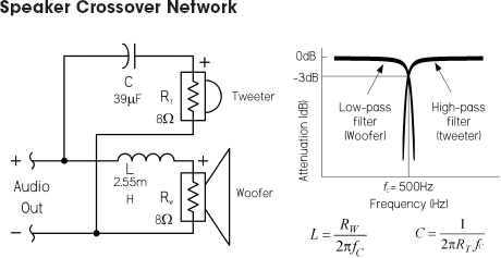
FIGURE 3.75 Crossover networks are used to provide each speaker in a system a range of frequencies most responsive to a given speaker’s dynamic range. For example, the circuit in the figure is a simple first-order crossover for a system including a tweeter (high-frequency dynamic) and woofer (low-frequency dynamic). To divert only high frequencies to the tweeter, a capacitor is placed in series with the tweeter, where the internal resistance of the tweeter and the capacitance form a high-pass RC circuit. A low-pass filter is used to pass low frequencies to the woofer. It uses an inductor in series with the woofer’s resistance. The response curves and formulas for calculating the cutoff frequency for each filter are provided to the right in the figure. Some popular crossover capacitors include polypropylene, polyester, and metallized-film capacitors.
3.6.12 Arc Suppression
There are two types of discharge that can damage switching contacts and generate noise in the process. The first is glow discharges, caused by the ignition of gases between contacts. These develop at around 320 V with about a 0.0003-in gap, and can be sustained at a much wider gap range. The other type of discharge is arc discharge, occurring at much smaller voltages, about 0.5 MV/cm. Minimum voltages and current are required for arc discharges to be sustained. Contact material also plays a role in sustained arc discharges (see table in Fig. 3.77).
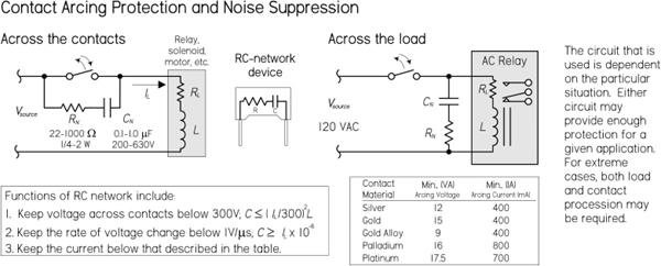
FIGURE 3.77
The main cause of discharge or arcing is the sudden switching off of an inductive load, such as a relay, motor, solenoid, or transformer. These inductive loads do not instantly let go of a current. At the instant a contact opens, the current through the contact does not want to change. When the switch is closed, the resistance is essentially zero, making the voltage zero, too. As the contact opens, the resistance increases, which leads to a high voltage that leads to the arcing or discharge effect across the contacts, usually destructive to contact life—it promotes contact erosion. See Fig. 3.77.
The role of the RC network, or snubber, is to keep the voltage across the contacts below 300 V, while keeping the rate of voltage change below 1 V/μs, as well as keeping the current below the minimum current levels specified for a particular switch contact material. See the table in Fig. 3.77. The capacitor acts to absorb the instantaneous voltage change. When the contacts are closed, the capacitor doesn’t play a role. As the contacts open, any change in voltage is restricted by the capacitor if its value is large enough to restrict the voltage change to less than 1 V/μs. However, a capacitor alone is not a good idea. When the contacts are opened, the capacitor charges up to the supply voltage. As the contacts close, an inrush of current results, limited only by residual resistance, and damage may still result. For this reason, a resistor is connected in series with the capacitor. The voltage across the contacts when opened is equal to the load current × resistance (V = IR). It is recommended that V ≤ supply voltage. In this case, the maximum resistance of the network will be equal to the load resistance.
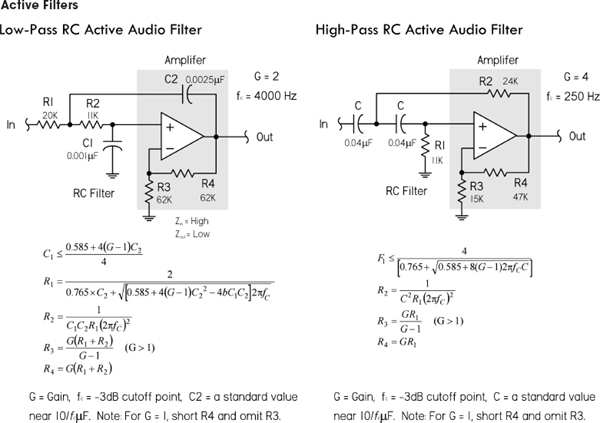
FIGURE 3.76 With the help of op amps, low-pass, high-pass, bandpass, and notch filters can be created with gain, if desired. Such filters are called active filters, since they have an active element (op amp), as opposed to being passive (no additional power source). The circuits in the figure are low-pass and high-pass active filters suitable for audio applications. The gain and desired cutoff frequency (-3 dB) can be obtained by using the provided formulas to calculate the component values. Polyester, polypropylene film, and metallized capacitors are good in filters at audio ranges.
Usually a 0.1- to 1-μF polypropylene film/foil or metallized-film capacitor with a voltage rating from 200 to 630 V will work for most applications. A carbon 22- to 1000-Ω, ¼- to 2-W capacitor is usually used for the resistance—the size and wattage depend on the load conditions. (In high-voltage applications, oil-filled capacitors with voltage ratings in the kilovolts are often used.) You can avoid building your own RC networks by simply buying prefab versions from the manufacturer.
Note that often shunt resistors, diodes, and gas discharge valves, along with various transient suppressor devices, can also be used to suppress arcing. However, some advantages RC networks have over these devices include bipolar operation suitable for ac application, relay operating time not very much affected, and no current consumption; electromagnetic interference suppression is also achieved (high-frequency EMI is present within the chaotic discharging sparks, but becomes dampened by the RC network).
In some ac circuits it may be necessary to connect the RC network across the load. For example, with ac relays, the relay contacts can also suffer from mechanical and electrical erosion due to arcing when subject to inductive spikes caused by sudden switching. Though diodes are used to suppress transients generated by dc relays, they cannot be used with ac relays due to the ac source’s dual polarity. The leftmost circuit in Fig. 3.77 shows an RC network connected across the ac relay to reduce arcing effects.
3.6.13 Supercapacitor Applications
The extremely high capacitance levels and low leakage rates of supercapacitors make them nifty devices in many low-energy supplies that require recharging in mere seconds. Many interesting solar-power circuits can be made, such as light-seeking robots that use solar energy stored in a supercapacitor to drive small motors. Usually in these circuits special energy-saving modulating circuits are used to pulse the motor in order to conserve energy. Figure 3.78 shows a few simple supercapacitor circuits to get you started.
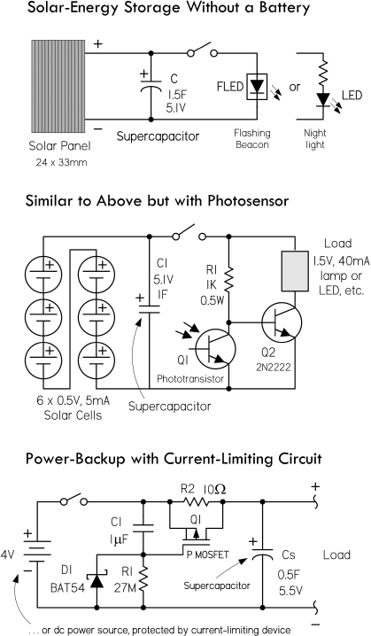
The circuit at the top in the figure uses a supercapacitor to store charge from a solar panel over time. The larger the capacitance, the more charge that can be stored and the more current that can be delivered to a load. Here, a simple flashing LED (FLED) is used as a nighttime beacon, getting its power from the supercapacitor charged during the day. Assuming the solar panel has fully charged C if C = 0.047 F, then FLED flashes for around 10 min when the light is removed or the switch is opened. If C = 1.5 F, then FLED flashes for hours. There are a number of other cool solar-powered circuits you can make, such as solar-powered engines and backup supplies. Though the circuitry is a bit more complex, they all basically use the same principle of energy storage shown here.
The second circuit is similar to the first, except now there is a phototransistor Q1 that keeps transistor Q2 off if exterior light exists. This prevents the supercapacitor C1 from discharging unless it’s dark. When it’s dark, Q1 turns off and Q2 turns on, providing approximately 10 s of illumination for one 40-mA, 1.5-V lamp. This can be used for short-term nightlights, for mailboxes, or near home entrances. This is a good circuit to avoid the hassle of dealing with dead batteries.
The circuit at the bottom uses a supercapacitor as a power backup for a battery (or a dc power source with current-limiting protection). As with the previous circuit, energy is stored in the supercapacitor; however, now a current-limiting regulator section is added to limit the current delivered to the supercapacitor when the power is first applied to the circuit. Thus, the supercapacitor can charge up without imposing a high current load on the battery. The MOSFET must be rated to dissipate the heat generated during the charging phase. This is a one-off event each time the device is turned on, which lasts only a few seconds, so the MOSFET doesn’t have to be rated to dissipate that amount of power continuously.
FIGURE 3.78
3.6.14 Problems
Problem 1: What do each of the following capacitor labels mean (see Fig. 3.79)?

FIGURE 3.79
Answer: (a) 0.022 μF ± 1%; (b) 0.1 μF ± 10%; (c) 47 pF ± 5%; (d) 0.47 μF, 100 V; (e) 0.047 μF ± 20%, −56% to +22% variation from +10°C to +85°C; (f) 0.68 nF; (g) 4.7 μF, 20 V; (h) 0.043 μF.
Problem 2: Find the equivalent capacitance and maximum voltage ratings for the capacitor networks shown in Fig. 3.80. Also, find V1 and V2 within circuit b.
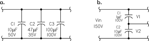
FIGURE 3.80
Answer: (a) 157 μF, 35 V; (b) 0.9 μF, 200 V, V1 = 136 V, V2 = 14 V.
..................Content has been hidden....................
You can't read the all page of ebook, please click here login for view all page.