
Chapter 8. The Operational Model
The tires hit the road; let the fun begin!
At this point, if you feel that you’ve earned your bread, here is some breaking news for you: The job ain’t yet done, my friend. Who will put your functional model into operation? I hear a familiar voice in the background calling out: “I rely on you to put this all into action. Let the tires hit the road!”
With a well-defined functional model, the components, once implemented, would need a home; that is, each of the components needs to run on a piece of hardware that is commensurate with the workload that the component has to support. While the functional model treated the system in terms of its usage (that is, who was using the system, how they were interacting with the system, and which components were used for the interactions), the operational model views the system in terms of its deployed context (that is, where the components are deployed and when they are invoked).
This chapter focuses on the operational model (OM) of a system. The OM defines and captures the distribution of the components in the IT System onto geographically distributed nodes, together with the connections necessary to support the required interactions between the components to achieve the IT System’s functional and nonfunctional requirements (NFRs); the purpose is to honor time, budget, and technology constraints. The chapter also focuses on how to iteratively build the operational model of an IT System through a three-phased approach starting with the logical operational model (LOM) and subsequently defining more specificities (elaboration) of the OM through two more views—the specification operational model (SOM) and the physical operational model (POM). Elaboration is an act of refinement that establishes increased accuracy and a greater degree of detail or precision.
The discipline of operational modeling is significantly expansive; it can get into the details of hardware architectures, into network topologies and architecture, or into distributed processing architectures. However, keeping to the central theme of this book, which is to focus on the essential ingredients and recipes to be a consistently successful software architect by defining just enough architecture artifacts, this chapter focuses on the elements of the OM that are essential for a software architect to understand to either be able to develop the OM on her own or to oversee its development. And yes, the chapter concludes by instantiating a subset of the operational model for the Elixir system case study.
Why We Need It
The goal of the operational model is to provide a blueprint that illustrates the appropriate set of network, server, and computational test beds necessary for the functional components to operate—not only individually but also supporting their intercomponent communications. The operational model helps in identifying and defining the
• Servers on which one or more of the functional components may be placed
• Compute capacity (memory, processors, storage) for each of the servers
• Network topology on which the servers are installed; that is, their locations, along with their intercommunication links
It is important to recognize and acknowledge the value of the operational model artifact of any software architecture; you can dedicate commensurate effort and diligence to its formulation only if you are convinced of its importance. I can only share with you the reasons that compel me to spend adequate time in its formulation:
Component placement and structuring—Functional components need to be placed on nodes (operational) to meet the system’s service-level requirements along with other quality requirements of the IT System; serviceability and manageability, among others. As an example, colocated components may be grouped into deployable units to simplify placement. Also, where required, the component’s stored data can be placed on a node that is separate from the one where the component itself is hosted. The OM maps the interactions (functional) to the deployable nodes and connections (operational). The operational concerns also typically influence the structuring of the components; technical components may be added and application components restructured to take into account distribution requirements, operational constraints, and the need to achieve service-level requirements.
Functional and nonfunctional requirements coverage—The logical- and specification-level views of the operational model provide details around the functional and nonfunctional characteristics for all elements within the target IT System, while the physical-level view provides a fully detailed, appropriately capacity-sized configuration, suitable for use as a blueprint for the procurement, installation, and subsequent maintenance of the system. The OM provides the functional model an infrastructure to run on; appropriate diligence is required to have a fully operational system.
Enables product selection—The blueprint definition (hardware, network, and software technologies) gets more formalized and consolidated through the incorporation of the proper product and technology selection. Some examples of hardware selection include deciding between Linux® and Windows® OS, between virtual machines and bare metal servers, or between various machine processor families such as the Intel Xeon E series versus X series. The technology architecture then becomes complete.
Enables project metrics—A well-defined operational model contributes to and influences cost estimates of the solution’s infrastructure, both for budgeting and as part of the business case for the solution. The choice of technologies also helps influence the types of skills (product specific know-how) required to align with the various implementation and deployment activities.
It is important to realize that the technical components, identified as a part of the operational model, must be integrated with the functional components. The operational model ensures that the technical architecture and the application architecture of a software system converge—that they are related and aligned. As an example, you can think of a business process workflow runtime server as a technical component (part of a middleware software product), yet it contains business process definitions and information about the business organization that are clearly application concepts. This component, therefore, has both application and technical responsibilities.
Just as with the functional model, it is critically important to acknowledge the value of the operational model as it relates to the overall architecture discipline. I intend to carry forward a similar objective from the functional model and into the operational model to illustrate the various aspects of the operational model and the techniques to develop and capture them.
Just take a step back and think about the power you are soon to be bestowed with—a master of both functional modeling and operational modeling!
On Traceability and Service Levels
The operational model is a critical constituent of the systems architecture, which connects many systems notes to form an architectural melody. In a way, the OM brings everything together. It is paramount that the IT constructs or artifacts that are defined must, directly or indirectly, be traceable to some business construct. In the case of the operational model, the business constructs manifest themselves in the form of service levels and quality attributes.
Quality attributes typically do not enhance the functionality of the system. However, they are necessary characteristics that enable end users to use an operational system relative to its performance, accuracy, and the “-ilities,” as they are popularly called—availability, security, usability, compatibility, portability, modifiability, reliability and maintainability. An understanding of the typical NFR attributes is in order.
• Performance—Defines a set of metrics that concerns the speed of operation of the system relative to its timing characteristics. Performance metrics either can be stated in somewhat vague terms (for example, “the searching capability should be very fast”) or can be made more specific through quantification techniques (for example, “searching of a document from a corpus of a 1TB document store should not exceed 750 milliseconds”).
• Accuracy and precision—Defines the level of accuracy and precision of the results (or outcomes) generated by the system. This is typically measured in terms of the tolerance to the deviation from the technically correct results (for example, “KPI calculations should remain within +/- 1% of the actual engineering values”).
• Availability—Determines the amount of uptime of the system during which it is operational. The most-talked-about example is when systems are expected to maintain an uptime SLA of five 9s, that is, 99.999 percent.
• Security—Defines the requirements for the protection of the system (from unwanted access) and its data (from being exposed to malicious users). Examples may include authentication and authorization of users using single sign-on techniques, support for data encryption across the wires, support for nonrepudiation, and so on.
• Usability—Determines the degree of ease of effectively learning, operating, and interacting with the system. The metric is typically qualified in terms of intuitiveness of the system’s usage by its users and may be quantified in terms of learning curve time required by users to comfortably and effectively use the system.
• Compatibility—Defines the criteria for the system to maintain various types of support levels. Examples may include backward compatibility of software versions, ability to render the user interface on desktops as well as mobile tablets, and so on.
• Portability—Specifies the ease with which the system can be deployed on multiple different technology platforms. Examples may include support for both Windows and Linux operating systems.
• Modifiability—Determines the effort required to make changes, such as new feature additions or enhancements, to an existing system. The quantification is usually in terms of effort required to add a set of system enhancements.
• Reliability—Determines the consistency with which a system maintains its performance metrics, its predictability in the pattern and frequency of failure, and its deterministic resolution techniques.
• Maintainability—Determines the ease or complexity measures to rectify system errors and to restore the system to a point of consistency and integrity; essentially adapting the system to different changing environments. The metrics are typically defined in terms of efforts (person weeks) required to recover the system from various categories of faults and also the system’s scheduled maintenance-related downtimes, if any.
• Scalability—Defines the various capacities (that is, system workload) that may be supported by the system. The capacities are typically supported by increased compute power (processor speeds, storage, memory) required to meet the increased workloads. Horizontal scalability (a.k.a. scale out) denotes the nodal growth (that is, adding more compute nodes) for a system to handle the increased workloads. Vertical scalability (a.k.a. scale up) denotes the need to add more system resources (that is, compute power) to support the increased workload.
• Systems Management—Defines the set of functions that manage and control irregular events, or other “nonapplication” events, whether they are continuous (such as performance monitoring) or intermittent (such as software upgrades—that is, maintainability).
There are definitely many other NFR attributes such as reusability and robustness that may be part of the system’s characteristics. However, in the spirit of just enough, the preceding ones are the most commonly used.
As a parting remark on service levels, let me add that you need to take SLAs very seriously for any system under construction. The SLAs are notorious for coming to bite you as you try to make the system ready for prime-time usage. SLAs are legal and contractual bindings that have financial implications such as fees and penalties. If you are not sure whether your system can meet the quantified SLAs (for example, 99.999 percent system uptime, available in 20 international languages, and so on), consider thinking in terms of service-level objectives (SLOs), which are statements of intent and individual performance metrics (for example, the system will make a best effort to support 99 percent uptime, pages will refresh at most in 10 seconds, and so on). Unlike SLAs, SLOs leave room for negotiations and some wiggle room; they may or may not be bound by legal and financial implications!
Developing the Operational Model
The operational model is developed in an iterative manner, enhancing the level of specificity between subsequent iterations, moving from higher levels of abstraction to more specific deployment and execution artifacts. The three iteration phases I focus on here are the conceptual operational model (COM), the specification operational model (SOM), and the physical operational model (POM).
The COM is the highest level of abstraction, a high-level overview of the distributed structure of the business solution represented in a completely technology-neutral manner. The SOM focuses on the definition of the technical services that are required to make the solution work. The POM focuses on the products and execution platforms chosen to deliver both the functional and nonfunctional requirements of the solution. The COM–SOM–POM story connotes that they ought to be developed in sequence, which, however, may not be the case. As an example, it may be completely legitimate to start thinking about but not fully develop the POM in the second week of a six-month OM development cycle. COM–SOM–POM deserves a little bit more page space to warrant a formal definition. A brief description follows:
COM—Provides a technology-neutral view of the operational model. COM concerns itself only with application-level components that are identified and represented to communicate directly with one another; the technical components that facilitate the communication are not brought into focus.
SOM—Transforms, or more appropriately augments, the COM view into and with a set of technical components. The technical components are identified and their specifications appropriately defined to support the business functions along with appropriate service-level agreements that each of them need to support.
POM—Provides a blueprint for the procurement, installation, and subsequent maintenance of the system. The functional specifications (from the functional model) influence and dictate the identification of the software products (or components) that are verified to support the relevant NFRs. The software components are executed on the physical servers (nodes). Software components collectively define the functional model; the set of physical servers (nodes) defines the physical operational blueprint.
These levels (or representations) of the OM typically evolve or are “elaborated” together during the development process, in much the same way as the functional model (see Chapter 7, “The Functional Model”).
Conceptual Operational Model (COM)
The COM is built out through a series of activities. The development of the COM is based on a few fundamental techniques: identify the zones and locations, identify the conceptual nodes of the system, place the nodes in the zones and locations, and categorize the placement of the nodes into a set of deployable units. The rest of this section elaborates on these techniques and activities.
For example, consider a retail scenario. I purposefully deviate from the banking example used in the earlier chapters; the retail scenario provides opportunities to address more variability as it pertains to the development of the system’s OM. The retail scenario, at a high level, is simplistic (on purpose). Users of this retail system can work in either offline or online mode. Users typically view inventories and submit orders at multiple stores. Two back-end systems—Stock Management System (SMS) and Order Management System (OMS)—form the core of the data and systems interface.
The development of the COM may be performed in four major steps:
1. Define the zone and locations.
2. Identify the components.
3. Place the components.
4. Rationalize and validate the COM.
Define the Zones and Locations
The first step is to identify and determine the various locations where system components (external or internal) are going to reside and from where users and other external systems may access the system. Zones are used to designate locations that have common security requirements. They are areas in the system landscape that share a common subset of the NFRs.
The recommendation is to adopt, standardize, and follow some notational scheme to represent OM artifacts. Keeping the notation catalog to a minimum reduces unnecessary ancillary complexities.
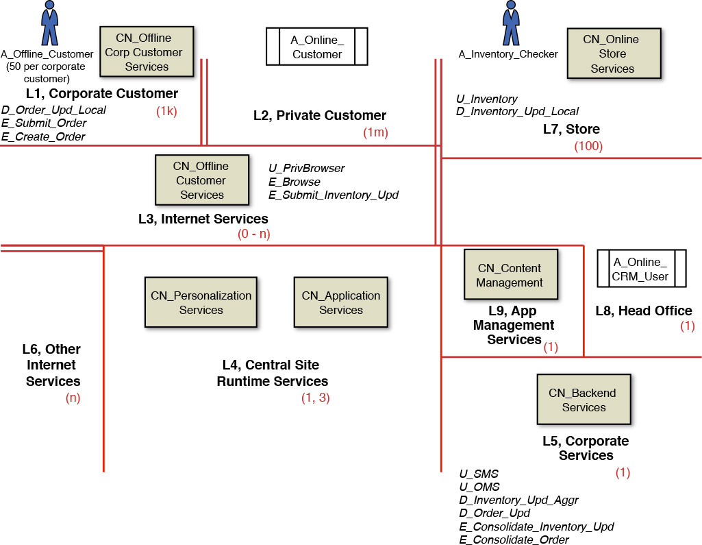
At a minimum, adopting a naming scheme to denote actors and system components is always beneficial. Artifacts (actors and components) in one zone may or may not have access to the artifacts in a neighboring zone. Some visual indicators that can assist in depicting interzone communication, or lack thereof, come in very handy; for example, double vertical lines between two zones indicate that interzonal communication is not allowed. The diagrammatic representation in Figure 8.1 depicts the locations and zones for an illustrative retail scenario.
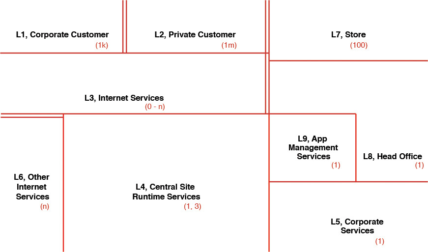
The figure shows different zones labeled as Lxx, <Zone Name> with a number in parentheses. Lxx refers to the standard abbreviation used to designate a unique location (xx is a unique number). The number in the parentheses denotes the cardinality. For example, L1 has a cardinality of 1,000, which implies that there could be up to 1,000 corporate customers (potentially distributed while similar in nature). A second example is L4, which has a cardinality of 1 or 3; a cardinality of 1 denotes the existence of only one data center instance (which will implicitly require 24/7 support), whereas having 3 instances implies that three data centers would support three geographies (a “chasing the sun” pattern). Notice that there are double lines between L1 and L2, whereas there is a single line between L4 and L6. The double lines provide a visual clue that the boundaries are strict enough to have no connection across the two zones that they demarcate. A single solid line, on the other hand, denotes that connectivity (for example, slow or high speed, and so on) exists across the two zones.
It is safe to state that architects introduce variances or extensions of the zonation depiction. However, the preceding simple principles would be good enough for a solution architect to illustrate the evolving operational model.
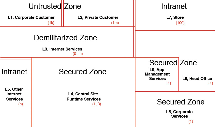
Zones can also be colored to denote the various access constraints and security measures that are applied to each one of them. The most commonly used enumeration of zones may be Internet, intranet, DMZ (demilitarized zone), extranet, untrusted zone, and secured zone. Figure 8.2 shows the categorization of these various zones as an illustrative example.
Identify the Components
A conceptual component node is used to denote a potential infrastructure node, which can host one or more application-level functional components. A conceptual component attributes the appropriate service-level requirements (a.k.a. NFRs) to the functional component (as developed in the functional model; refer to Chapter 7). The conceptual nodes may be identified by performing the following type of analysis:
• How different system actors interface with the system
• How the system interfaces with external systems
• How a node may satisfy one or more nonfunctional requirements
• How different locations may require different types of deployable entities
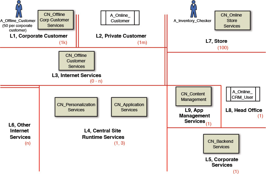
Networking artifacts—for example, LANs, WANs, routers, and specific hardware devices and components (for example, pSeries, xSeries servers)—do not get identified as conceptual components. In other words, a conceptual component node provides a home for one or more functional components on the deployed system. Figure 8.3 shows a set of conceptual components along with a set of actors and how they are distributed into different zones in the COM.
Place the Components
The most significant challenge in bringing the functional model and operational model together is the placement of the functional components on the operational model. While it is technically possible to place the components directly, doing so often is far more difficult. Wouldn’t it be good to have some technique to introduce some formalism to bridging the proverbial functional-operational model gap? Deployable units could be the answer; see Figure 8.4. (Refer also to the “Deployment Operational Models” [n.d.] article.)
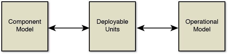
Figure 8.4 Deployable units are typically used to bridge the gap between the functional model and the operational model.
Note: The component model in Figure 8.4 contains the “functions” (refer to Chapter 7 for more details).
And just when you thought that your repertoire might be full, allow me to introduce yet another categorization scheme; this one is for the deployable units! Deployable units (DU) come in four flavors: Data Deployable Units (DDU), Presentation Deployable Units (PDU), Execution Deployable Units (EDU), and Installation Deployable Units (IDU):
• DDU—Represent the data that is used by the components to support a given behavior or function; it is the place where data is provisioned. Some of the aspects of the data worth considering include the volume of the data, frequency of data refresh, data archive and retention policies, and so on.
• PDU—Represent the various techniques through which access needs to be provided to harness the functionality of a component. It supports the interface of the system to external actors (real users on devices such as laptops and handhelds) and systems.
• EDU—Focus on the execution aspects of a component, for example, compute power needs (processor speeds, memory, disk space), frequency of invocation of the component, and so on.
• IDU—Focus on the installation aspects of a component. Examples include configuration files required for installation, component upgrade procedures, and so on.
To keep matters simple, it is okay for solution architects to focus on the DDU, PDU, and on some aspects of the EDU. Keep in mind that the complete development of the OM definitely requires a dedicated infrastructure architect, especially for nontrivial systems. The techniques outlined in the following sections allow you to get a good head start on the OM while being able to talk the talk with the infrastructure architect as you validate and verify the operational model for your system.
Let’s spend some time on some of the considerations while placing the different types of DUs. Placement starts by assigning xDUs (x could be P, D, or E) to the conceptual component nodes (CNs).
Place the Presentation Deployable Units (PDU)
The types of users (that is, the user personas in a location) provide a good indicator to the type of presentation components required for the user to interface with the system. A rule of thumb here could be to assign a PDU for each system interface. Such a PDU could support an actor either to the system interface or to an intersystem interface.
To provide some examples (refer to Figure 8.3), you can assign a PDU called U_PrivBrowser to the CN_Online_Customer_Services component through which the A_Online_Customer actor can access the system features. Similarly, you can assign U_Inventory to CN_Online_Store_Services, U_SMS and U_OMS to CN_Backend_Services, and so on. Figure 8.6 shows a consolidated diagram with all the PDUs placed on the COM.
Place the Data Deployable Units (DDU)
Having the placement of DDUs follow that of the PDUs makes the job a bit easier; it becomes easy to figure out which PDUs need what data. However, the placement of the DDUs gets a bit more tricky and involved.
In the retail example, it is quite common to have orders submitted both in online as well as in offline mode. Each local store also requires that its inventory records be updated. Not only the inventory needs to be updated locally, but also the central inventory management system requires updating. As you can see, it is important for data to not only be updated locally (inventory) and temporarily stored (submitted orders), but also to be updated in the back office; that is, the back-end services. The DDUs need to support both forms. As such, a data entity may require multiple types and instances of DDUs. For example, an Inventory business entity may require a DDU per store (let us give it a name: D_Inventory_Upd_Local) supporting the local update in each store location and also a single DDU (let us give it a name: D_Inventory_Upd_Aggr) that aggregates the updates from each store-level DDU and finally updates the master inventory system in the back office. Submitted orders typically follow the same lineage; that is, they could be stored locally (let us give it a name: D_Order_Upd_Local) before they are staged and updated into the central order management system (let us give it a name: D_Order_Upd) once a day or at any preconfigured frequency. Figure 8.6 shows the consolidated diagram with all the DDUs placed on the COM.
Other variations to the DDU also may be considered. For example, a customer relationship management (CRM) system can have data entities that are not too large in volume and do not change very frequently, so there is a possibility to hold them in an in-memory data cache. In the same CRM, other data entities can be highly volatile and with very high transactional data volumes; they may require frequent and high-volume writes. Data, along with its operational characteristics, dictates its rendition through one of the types of DDUs. To summarize, a catalog of data characteristics may need to be considered while determining the most appropriate DDU. Some of the following characteristics are quite common:
• Scope of the location where the data resides; for example, local storage or centralized storage
• Volatility of the data; that is, the frequency at which the data needs to be refreshed
• Volume of the data being used at any given instance; that is, the amount of data used and exchanged by the application
• Velocity of the data; that is, the speed at which data enters the IT System from external sources
• Lifetime of the data entity; that is, the time when the data may be archived or backed up
Don’t assume that all business or data entities end up with the same fate of being instantiated through multiple deployable units. Some easier ones have a single place where all the CRUD (create, read, update, delete) operations are performed. So do not panic!
Place the Execution Deployable Units (EDU)
The identification of the PDUs and DDUs is a natural step before we turn our attention to the placement of the EDUs. There are a few choices available for placing the EDUs: “close to the data,” “close to the interface,” or both (which implies that we split the EDU).
Colocating execution and data is clearly the default option, thereby acknowledging the affinity between data and the application code that is the primary owner of the data (see Chapter 7). So, in many circumstances, this will probably be the easiest and apparently the safest choice. If the business function demands highly interactive processing with only occasional light access to data, it may be appropriate to put the execution nearest to the end user even if the data is located elsewhere (perhaps for scope reasons). It is very important to note that the commonality of service-level requirements of multiple components may dictate the consolidation of their respective EDUs into a single EDU.
In the retail example, the EDU E_Submit_Inventory_Upd is placed close to the conceptual component called CN_Online_Store_Services; that is, the local stores from where such updates are triggered. A related EDU called E_Consolidate_Inventory_Upd is placed close to the data; that is, close to the CN_Backend_Services conceptual component that resides at the back office. Similarly, E_Create_Order is placed close to the interface, while E_Consolidate_Order is placed close to the CN_Backend_Services conceptual component. On the other hand, E_Browse is an EDU that is placed close to the PDU where the inventory is browsed by the offline and online customers. Figure 8.6 shows the consolidated diagram with all the EDUs placed on the COM.
It is important to recognize that the intent of illustrating the retail example without providing too many in-depth use cases is to provide guidance on how a typical COM may look; I chose relatively self-descriptive names for the CNs in the example (refer to Figure 8.3) so that you can more easily comprehend their intent. The COM for your project-specific OM may look very different.
Note: The terms conceptual component and conceptual node are used interchangeably.
Having placed all the deployable units, we can turn our attention to the interactions between the various deployable units. From the PDU <-> EDU & DDU <-> EDU matrices, we can infer the inter DU interactions.
It is important to note that
• Interactions occur between DUs that have been placed on conceptual nodes.
• You are primarily interested in the interactions between DUs that have been placed on different nodes.
• In some situations, you also need to keep track of interactions between DUs placed on different instances of the same conceptual node (for example, if DUs placed on the CN in L3 interact with the same DU placed on the same CN but located in one of the different L3 instances). Note that you can have more than one instance of L3.
Interactions provide great clues on the placement of the EDUs. As a case in point, consider a slight variation of the retail example such that the data needs to be held centrally (in the back office), as shown in Figure 8.5. Also, assume that it was decided (maybe for reasons of scope) to hold the attributes of a component centrally (labeled as HQ in Figure 8.5), represented by the data deployable unit D3. And further, this example also has distributed users who need access to this data (through their appropriate presentation component, U1), via the execution component P3.
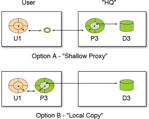
How do you link these deployable units?
Of the many options, let’s consider the following two:
1. In the first option, P3 is colocated with D3 on the HQ component node, and a “shallow proxy” technical component, which is on the User component node, acts as a broker between the components U1 and P3. This is a fairly normal arrangement in architectures in which distributed computing technologies (for example, CORBA or DCOM object brokers) may be used.
2. In the second option, P3 is colocated with U1, and some form of middleware is used to fetch the necessary attributes of the required components from D3 “into” P3. This is also a fairly normal arrangement, although at the time of this writing, it usually relies on bespoke (custom developed) middleware code.
Which of these two options is better? Although you can quickly start with the standard consulting answer “It depends,” you may need to qualify and substantiate the classic cliché with the fact that the choice should be informed and influenced by the operational service-level requirements and characteristics that are required to be met. Let’s look at some of the strengths and weaknesses of each of the two options.
Option 1 (shallow proxy):
Strengths:
• Response times between U1–P3 interactions should be fairly consistent.
Weaknesses:
• As the requirements placed on the shallow proxy middleware grow, system management may become more complex.
• Response times may be long, particularly if interactions between U1 and P3 need to traverse slower networks or require multiple network hops.
Option 2 (local copy):
Strengths:
• Following the initial fetch of attributes, response times may be quick.
Weaknesses:
• “Roll your own” (custom) middleware code may require significant code management.
• Initial response time, while fetching attributes, may be long, particularly over slower, constrained networks.
As is evident from the preceding descriptions, often multiple placement options exist; the service-level requirements or agreements and the technology considerations often dictate the most appropriate choice.
Getting back to the retail example (a representative COM for the retail scenario example), the COM may look like Figure 8.6.
Note: The deployable units are shown in italic in Figure 8.6.
Rationalize and Validate the COM
Before you call the COM complete, one suggestion, if not a mandate, would be to validate the COM. First of all, you should have a good feeling of what you have developed so far and for which you can use some sniff-test techniques. For starters, does it have the right shape and feel? For example, some of the litmus test verification questions you should be asking include: Is the COM implementable using available technology? Is the degree of DU distribution adequate to realize the NFRs? Are the cost implications of meeting the NFRs reasonable (budget, cost benefit analysis)? And finally, if the COM passes these tests to your degree of satisfaction, I recommend one last step: to walk through some of the carefully selected architecturally significant use case scenarios. Such walkthroughs provide a powerful mechanism of verifying the viability of the operational model. Figures 8.7 and 8.8 provide a pictorial representation of a walkthrough for the retail scenario.
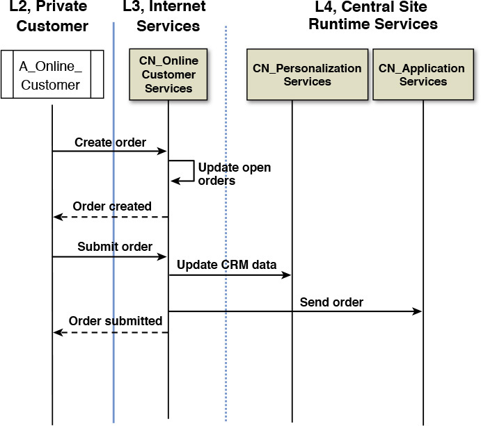
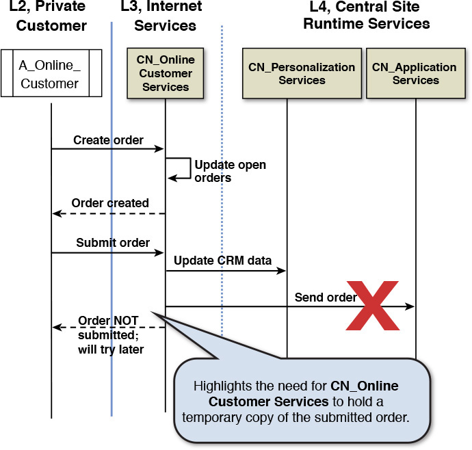
Figure 8.8 Walkthrough diagram highlighting the capability of handling error conditions and also some design decisions.
Although we spent quite a bit more time than usual on one section, the idea is to have a solid understanding and appreciation for the COM such that the SOM and POM will be easier to comprehend. More importantly, as a solution architect, you will be more involved in the COM, and once it is commensurate with what your system needs are, you can delegate the ownership of developing the SOM and POM to your infrastructure architect!
Specification Operational Model (SOM)
The specification operational model (SOM) identifies and defines the technical services and their specifications required to make the solution work with the same key objective: the solution meets all the nonfunctional requirements. So, while the COM gave a shape and feel to the operational model, the SOM enables the COM to put on its shoes and go for a run, so to speak—by identifying and defining a set of technical services that take one step forward toward instantiating the runtime topology. And although this chapter covers the most commonly needed aspects of extended operational modeling, it is important to acknowledge that the activities outlined in this section, for the SOM, provide the basis of many specialized subject areas in operational modeling, namely:
• Developing a security model
• Analyzing and designing the process and technologies for system availability
• Planning for elasticity and system scaling
• Performance modeling and capacity planning
Developing the specifications for the technical services and components is about answering questions: How will the COM be instantiated? What are the IT capabilities of each part of the system that are required to make it work? and so on. The main focus is on the infrastructure components—defining their specifications required to support and instantiate the COM. Although the technical specifications are developed in a product- and vendor-independent manner, their development drives the selection of the infrastructure products and physical platforms. It also defines how the application-level DU placement strategy will be supported technically: how to ensure maintaining distributed copies of data at the right level of currency; how to achieve the required levels of transaction control or workflow management, and so on. And similar to the COM, an infrastructure walkthrough ensures validation and completeness. Collection of the technical services and their associated components provides a view of the runtime architecture of the system—the nodes and connections that have to be defined, designed, developed, and deployed. The SOM is expected to provide the IT operations personnel with valuable insights into how and why the physical system works the way it does.
The development of the SOM may be performed in three major steps:
1. Identify specification nodes.
2. Identify technical components.
3. Rationalize and validate the SOM.
Identify Specification Nodes
The initial focus is to determine the specification nodes (SNs). The determination process starts by examining the catalog of CNs and grouping them by similarity of their service-level requirements. In the process, CNs may undergo splitting such that various types of users, with different service-level needs, may be accommodated. To be explicit, the deployable units (PDU, DDU, EDU) may need to be rearranged; that is, split, consolidated, or refactored. It may be interesting to note here that, although the functional model focuses on identifying subsystems by grouping functionally similar components, the operational model focuses on identifying specification nodes by grouping components by service level requirements.
On one hand, I am saying that the DUs may be split or refactored, while on the other hand, I am suggesting a consolidation of CNs based on their proximity of service-level requirements. Confusing, huh? You bet it is! Let me see if I can clarify this a bit using an example.
In the retail example, consider the requirement that users are split between using mobile devices and workstations; that is, some users use the mobile devices to place orders, whereas some others typically use their workstations for interfacing with the system. To support both user communities, you may split the PDU and EDU components for customer order creation. The PDU is split into two DUs and placed on two separate SNs (SN_Create_Order_Mobile and SN_Create_Order) for mobile device users and desktop users, respectively. The EDU is split between one that accepts user input from the mobile devices (SN_Order_Accept_Mobile), a second that accesses data from the desktop users (SN_Order_Accept), and a third that accesses the data from the back-end systems (SN_Order_Retrieve). You can think of the identified SNs as virtual machines, on each of which various application-level components are placed. Each identified SN may need installation DUs for installing and managing the various application components that it hosts.
In summary, in the process of identifying the SNs, we end up playing around with the catalog of DUs, assessing their commonalities relative to the various NFRs (response time, throughput, availability, reliability, performance, security, manageability, and so on) and end up splitting or merging the DUs to place them on the SNs to ensure that the various NFRs are met.
Identify Technical Components
The focus of this step is to augment the SN catalog with any other required nodes and identify the set of technical components required to satisfy the specified service-level agreements.
The SNs identified in the previous step are primarily derived from the DUs, along with the NFRs that are expected to be met. You need to ensure that the identified SNs can communicate between each other (that is, the virtual machines have established connectivity) and which new SNs (for component interconnections, among other integration needs) may be identified. Subsequently, you need to identify technical components that will support the implementation of the identified SNs and their interconnections. It is important to note that, since any SN may host multiple DUs and components, both the intracommunication between components within an SN and the intercommunication between SNs would require commensurate interconnectivity techniques to meet the service-level requirements. This may necessitate additional SNs to be introduced, for example, to facilitate the interactions.
Let’s look at an example. In the retail example, consider intercommunication between components in the store locations and the back office. Some of the data exchange may be synchronous and mission critical in nature to warrant a high-throughput subsecond response communication gateway (identified as SN_Messaging_Mgr). On the other hand, some other usage scenarios can work with a much more relaxed throughput requirement, and hence, asynchronous batch transfer (identified as SN_File_Transfer_Mgr) of data may well be a feasible and cost-effective option. As you can see, a single conceptual line of communication, between the store location and the back-end office, could need two different technical components to support the intercommunication between the SNs. Network gateways, firewalls, and directory services (SN_Access_Control) are some examples of technical components that directly or indirectly support the business functions.
Technical components address multiple aspects of the system. Some technical components directly support the DUs (the presentation, data, and execution). Other types of technical components address system aspects such as the operating systems, physical hardware components (for example, network interfaces, processor speed and family, memory, and so on) for each of the SNs, the middleware integration components bridging the various DUs (for example, message queues, file handlers, and so on), some systems management components (for example, performance monitoring, downtime management, and so on), and some application specific components (for example, error logging, diagnostics, and so on). It is noteworthy how different types of technical components address different system characteristics. As examples, the middleware integration components are attributed with protocols and security they support, along with data exchange traffic and throughput metrics; the systems management components determine planned system downtime and systems support, and the hardware components determine the scalability potential of the system and various means to achieve them.
The integration components and the various connection types (connecting the components) carry key attributes and characteristics that address the system NFRs. The following attributes of system interconnects provide key insights:
• Connection types—Synchronous or asynchronous modes of data exchange
• Transaction—Smallest, largest, and average size of each transaction
• Latency—Expected transmission times for smallest, largest, and average size transactions between major system components
• Bandwidth—Capacity of the network pipe to sustain the volume and latency expectations for the transactions
The identification of the technical components provides a clearer picture of the hardware, operational, communications, and systems management characteristics of the system—aspects that serve as key inputs to the POM!
Rationalize and Validate the SOM
The proof of the pudding is in the eating, as the adage goes, and SOM activities are no exception to that rule! It is important to pause, take a step back, and assess the viability (technical, cost, resources, timeline) of the SOM as it pertains to the solution’s architecture. Here, you use the same technique used while developing the COM to assess the viability: scenario walkthroughs to ensure that the normal and failure conditions can be exercised while meeting the nonfunctional requirements and the desired service levels.
The technical viability assessment of the SOMs may consider, but is not limited to, the following aspects:
• Characteristics of the included DDUs—Volume, data types, data integrity, and security
• Characteristics of the included EDUs—Response time latency, execution volumes, availability, transaction type (batch, real time)
• System integrity—Transaction commits or rollbacks to previous deterministic state of the system
• Distribution of data across multiple SNs in various zones and locations—Is it commensurate with required transactional integrity and response times?
The intent of the technical viability assessment is to validate that the SOMs will support the service-level requirements and support the architecture decisions that primarily address the system’s NFRs.
Let’s take an inventory of some of the SNs that we identified, in our retail example, as we walked through a portion of the system:
• SN_Create_Order_Mobile—A virtual machine that encapsulates the presentation-level CNs that orchestrate the collection of order details from a mobile device.
• SN_Create_Order—A virtual machine that encapsulates the presentation-level CNs that orchestrate the collection of order details from any desktop machine.
• SN_Order_Accept_Mobile—A virtual machine that encapsulates the execution-level CN that triggers and processes the order creation business logic from a mobile device.
• SN_Order_Accept—A virtual machine that encapsulates the execution-level CN that triggers and processes the order creation logic from any desktop machine.
• SN_Order_Retrieve—A virtual machine that works in conjunction with the SN_Order_Accept_Mobile and SN_Order_Accept nodes to send and retrieve order details from the order management system that resides at the back office.
• SN_Messaging_Mgr—A technical component that supports high-speed, low-latency, asynchronous data transfer between the store locations and the back office.
• SN_File_Transfer_Mgr—A technical component that supports relatively (to SN_Messaging_Mgr) lower-speed, higher-latency, batch mode of data transfer between the store locations and the back office.
• SN_Access_Control—A technical component that enables user authentication and authorization along with other policy-driven security management.
• SN_Systems_Mgmt_Local—A technical component that implements systems monitoring and management at each store location, one per store location.
• SN_Systems_Mgmt_Central—A technical component that implements systems monitoring and management functions at the back office.
• SN_Data_Services—A technical service at the back office that functions as a data adapter, abstracting all access to the system’s one or more databases.
• SN_Order_Management_Services—A set of technical services that expose the functional features of the order management system.
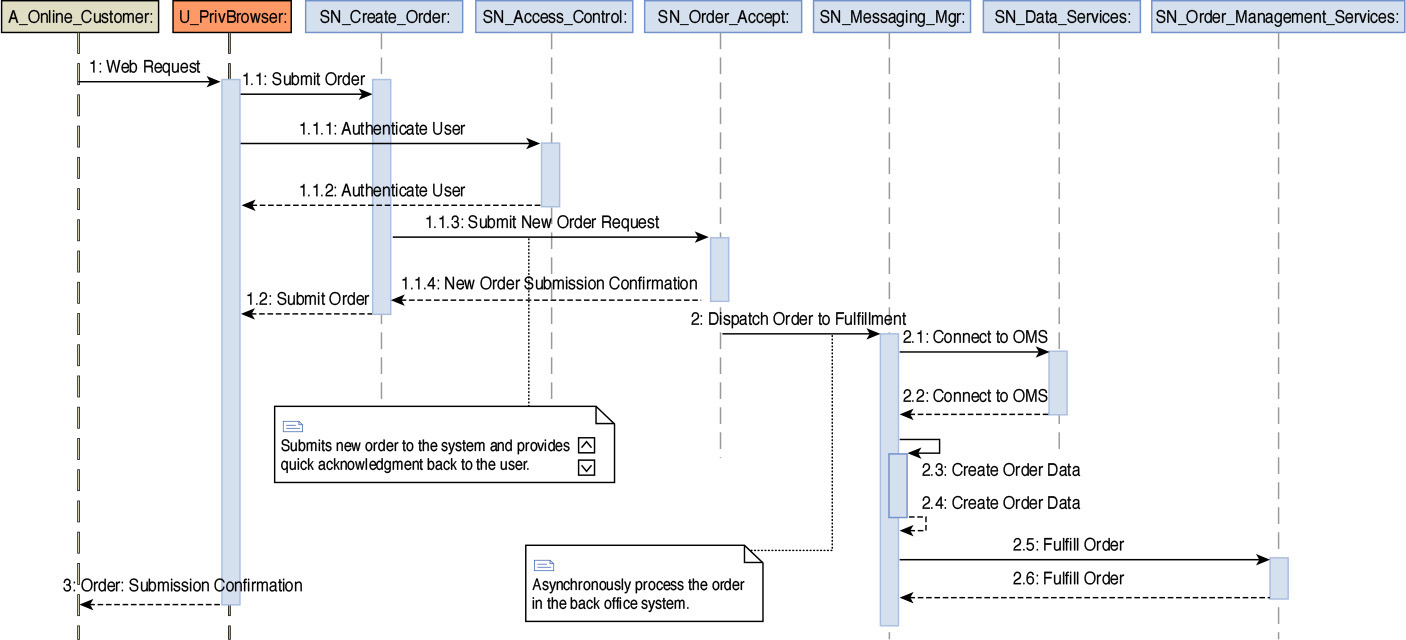
As a part of the validation activities, a step-by-step walkthrough of a set of sequence diagrams is recommended (see Figure 8.9). It is, however, important to take note of the fact that not all use cases must be illustrated by sequence (walkthrough) diagrams during the SOM elaboration phase; only the architecturally significant use cases should be walked through. This further highlights the fact that, as a practical measure, it is important to focus on the use cases that are architecturally important and foundational to drive the system’s overall architecture and blueprint.
To summarize, the activities of the SOM focus on the placement of the solution’s application and technical components—that is, the CNs, compute (storage, processor, memory), installation units, middleware and external presentation function, onto specified nodes together with the identification and placement of the communications and interactions between the specified nodes. This is done so that the system can deliver the solution’s functional and nonfunctional requirements, including consideration for constraints such as budget, skills, and technical viability.
And just to be clear, unless you are climbing up the infrastructure architect ranks to your newfound high ground as the solution architect, you will typically delegate the elaboration and completion of the SOM to your infrastructure architect while you focus on the bigger picture; that is, the other critical aspects of your overarching solution architecture. This should either give you comfort (if you are an infrastructure architect to begin with) or relief (for being able to establish the foundation and then delegate) to be able to move on!
Physical Operational Model (POM)
The physical operational model (POM) focuses on making the appropriate technology and product choices to instantiate the SOM and hence to deliver the required functionality and expected service levels. It is used as a blueprint for the procurement, installation, and subsequent maintenance of the system. The creation of the POM involves taking decisions that tread a fine balance between three conflicting forces—feasibility, cost, and risk—as they relate to the realization of the requested capabilities. It is not uncommon to see that the outcome of the feasibility-cost-risk triage results in making compromises (postponement or severance) on the functional and nonfunctional capabilities for a less risky or a more cost-effective solution.
The POM may be developed in three major steps:
1. Implement the nodes and connections.
2. Ensure meeting the Quality of Service (QoS).
3. Rationalize and validate the POM.
Implement the Nodes and Connections
The focus of this step is to select the most appropriate hardware, software, and middleware products that collectively meet the functional and nonfunctional requirements of the system.
The selection of the infrastructure components (hardware, software, middleware, and networks) is often nontrivial in nature, primarily owing to the multiple factors that influence the selection process. Let me share my experience with some of the most common questions and considerations that typically influence the selection and decision-making process:
• The maturity of the product in the marketplace—Often, however promising a marketing brochure touts a new product, it is wise to avoid adopting early versions of the product. (Let someone else be the guinea pig of something new! We frequently get enamored with the “shiny toy” syndrome.)
• The extent to which a product meets the required functional specifications—The product’s ability and its proven track record to integrate with other chosen products (for the system) should be considerations.
• The physical topology required to install and configure the product—As an example, some products are easy to install and configure, and they can work in both on-premise data centers as well as in cloud data centers. Some others, such as purpose-built hardware appliances, may not be as easily installable on cloud data centers as they are on traditional data centers.
• The roadmap of the product along with the stability and experience of the product vendor—Some product vendors may not have adequate regional establishments for product maintenance and support. A vendor’s strategic roadmap of maintaining and enhancing the product’s vitality and capabilities is also a key consideration (for example, a product may be close to its end of life). We must also assess and validate the track record of the product being productively used in specific industry domains of interest.
• The enterprise architecture blueprint and the company guidelines—An existing enterprise architecture blueprint drives a set of guidelines around the usage of some products in the context of the existing enterprise landscape. Vendor relations also drive explicit or implicit company guidelines around vendor preferences. It is quite common to come across situations in which a company, for example, is already vested in an all-IBM product portfolio; in such cases, considering a non-IBM product may be a difficult sell and also may introduce additional technology integration challenges.
• The hardware infrastructure required to install the product to support the nonfunctional requirements—Some products can scale vertically quite easily (adding more memory, using faster processor family and storage), whereas some may require a quicker adoption of horizontal scaling to achieve the required scaling needs (adding more servers and product instances). Cost implications, typically, are heavily influenced by scaling needs.
The selection process, as you can see, may turn out to be quite complex and time consuming. You have to be on a continuous and proactive lookout for opportunities to simplify and accelerate the selection process. My eyes usually light up when I spot opportunities to embrace the theories of natural selection. Following are some opportunities that I have come across:
• Identify the givens, policies, vendor preferences, and rules for qualification in a given enterprise. This certainly reduces the coverage area where you need to cast your net and reduces the frustration of product acquisition and procurement.
• Leverage past experiences where a product has worked great in a similar industry and functional landscape.
• Assess how preselected products may influence the rest of the selection process. For example, stay with one vendor product portfolio to ease integration challenges and vendor support. This way, you can identify the source of any problems.
Think you have enough information for you to oversee the product selection process? As the overall enterprise architect, I certainly would consider myself to be equipped enough at this point. I could ensure that the proper process and techniques are in place to not only assist the infrastructure architect to formalize the product selection but also for me to be able to review and validate the outcome.
And just when you thought that this step was complete, I have to remind you that we have not yet worked on the connections! How would these selected products communicate with each other? How may products need to be connected and in how many locations? Are the connections identical in all locations, or do they vary based on nonfunctional needs or network bandwidth limitations, among other factors?
Let’s consider the retail example for a moment. The COM identified a set of zones and locations along with a set of logical nodes that were placed in each of the zones. The functional needs determine the connectivity between the logical nodes to satisfy one or more use case scenarios. The nonfunctional needs drive the nature and mode of data exchange—for example, request-response versus asynchronous batch data delivery.
The realm of connections and their design and implementation squarely fall under the purview of a network architect—one who lives and breathes in the world of LANs, WANs, MPLS, routers, and switches. As the enterprise architect, you need to understand the rationale of the design and buildout of the network topology that supports the connections required for the system to be operational.
It is important to empower the network architect with the required NFRs that need to be supported, along with the various architecture alternatives for data exchange between various nodes. The “exchange between various nodes” provides a clue that, in order to come up with a commensurate network topology, it is critical to formalize a node-to-node connectivity matrix. The quest for such a connectivity matrix begins!
I have typically employed some matrix computation techniques to develop the node-to-node connectivity matrix that I elaborate on in the rest of this section. It requires you to have some basic knowledge of linear algebra (specifically of matrix manipulations). You may choose to skip the rest of this math-heavy section. If you take away nothing else from the mathematical treatment, at least understand the following essence:
You need to understand not only how each node is connected to each other but also the relative strengths of the connections. For example, a node N1 may be connected to another node N2 and the relative weight of the connection may be 3. N1 may also be connected to N3 with a relative weight of 2 and to N4 with a relative weight of 5; N2, on the other hand, may be connected only to N1. In such a scenario, it is evident that the network that connects N1 to the rest of the nodes in the operational topology would need to be more robust and support a higher bandwidth than the network that is required to connect N2 to the rest of the system.
The purpose of the matrix algebra manipulations in this section is to come up with a mathematical technique to aid in such a derivation.
To make matters comprehensible, you might find a little refresher on matrix algebra helpful (see the “Matrix Algebra” sidebar).
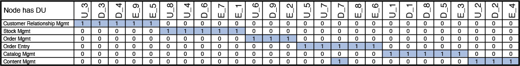
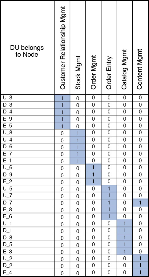
So, let’s apply a bit of matrix algebra. The goal is to find out how each node is connected to the rest of the nodes and also to get a sense of the relative weight of the connections. A node, in this discussion, represents a physical server that hosts and runs one or more middleware components or software products. From the COM, you get a clear picture of the interconnectivity between the DUs.
Let A denote the DU accesses DU matrix. You have already done the hard work of placing DUs on nodes when developing the SOM. Let B denote the Node hosts DU matrix (that is, nodes are the rows, and the DUs are the columns). Let’s introduce a third matrix that represents DU belongs to Node; this is nothing but the transpose of the B matrix (that is, DUs are the rows, and the nodes are the columns). The goal is to find the representation of Node is connected to Node matrix in which the value in each cell will provide a good representation of the expected relative strengths for each of the internode connections. To formulate the representation of how nodes are connected to other nodes; that is, the Node is connected to Node matrix representation, you need to apply some smart matrix manipulations (see the “Matrix Manipulation for Node-Node Connectivity” sidebar).
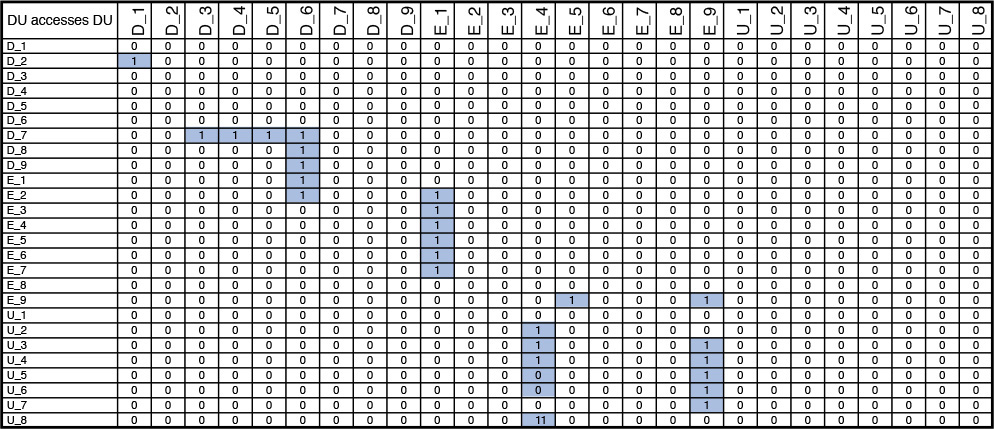
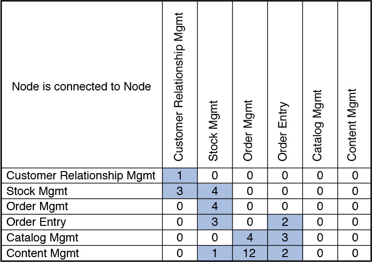
Referring to the Y matrix in the “Matrix Manipulation for Node-Node Connectivity” sidebar, the values in each cell signify the strength of a specific node-node pair communication or interaction.
The network architect is well positioned to take it from here. The weights of each interconnection, between the nodes, will be a key input in the final determination of the bandwidth requirements. The locations, zones, frequency, and volume of data exchange, along with the physical deployment topology of the products and application components, will also serve as key inputs to determine the network topology and its physical instantiation.
So, although you would, in all possibilities, require a dedicated network architect to finalize the network infrastructure, enough information and guidelines have been developed here to aid the validation of how the connections will be physically implemented and also testify to their adequacy to support the nonfunctional and service-level requirements of the system.
Ensure Meeting the Quality of Service (QoS)
The previous step ensures t hat the physical operating model is defined: the products and technologies chosen, along with the network layout and infrastructure required to connect the products together to support not only the required functionality but also most of the NFRs.
This step focuses on refining the configurations of the products, technologies, and networks so that some key NFRs—for example, performance, capacity planning, fault tolerance, and disaster recovery, among others—may also be addressed. An entire book can be written on QoS; this chapter focuses only on some of the important concepts that a solution architect would need to recognize, understand, and appreciate so that she can better equip herself to work with the infrastructure architect while formalizing the POM.
System performance is a critical metric, the satisfaction of which is imperative for the system’s ultimate users to accept and be happy with using it. Performance describes the operating speed of the system; that is, the response of the system to user requests. QoS, in the context of performance, should define, in a deterministic manner, how the system maintains or degrades its ability to keep up with the performance benchmarks in the event of increased system workload. What happens when the load on the system increases?
First of all, what defines increased load? Think about a system that is operational. Each time the system is running, it may generate new transactional data. This data would be stored in the persistent store; the volume of generated data will increase with time. A system’s ability to maintain the latency of the same database queries on a 5GB database versus on the same database that increases to, say, 1TB is an example of the system’s ability to maintain its performance with increased system workload.
In another example, the number of users who are exposed to using the system may also increase with time; the number of concurrent users accessing the user interface may well be on the rise. The system’s ability to maintain latency by generating or refreshing its user interface when 10 concurrent users access the system versus when 125 users access the same user interface is a measure of the system’s performance capabilities. In fact, there is a very fine line between a system’s performance and its scalability. Scalability defines how a system can keep up with increased workload while either maintaining its performance measures or degrading it in a deterministic manner.
Scalability is usually described and defined (as well as implemented) in two ways: horizontal and vertical. Stated simply, horizontal scalability applies various techniques to align the infrastructure with system needs, by adding more machines (that is, servers) to the pool of resources, also called scale out. Vertical scalability applies various techniques to align the infrastructure with system needs, by adding more compute power (that is, processors, memory, storage) to the existing pool of resources, also called scale up. In scale-out architectures, you can partition the data and also apportion the workload into multiple servers in the resource pool and enforce true parallelism and pipelining if architected correctly. Such architectures allow the system to address fault tolerance; that is, the system is able to function even in the event that one resource is down (that is, the second set of resources, supporting the same functions, will take up the workload). In scale-up architectures, you can apportion the workload only to different cores (that is, processor and memory), all within the same server resource.
The one downside of a scale-up technique is that you are putting all your eggs in one resource (server) basket. If it fails, your system is down. Additionally, in the event that, once you hit the upper limit of scaling up and still the system is not able to meet the performance expectations, you have to start thinking of changing the infrastructure architecture from scale up to scale out; in other words, you need to start adding new resources (servers) to the pool. The scale-out architecture, although much more robust and extensible by its very nature, comes with its own set of challenges: the cost of additional server resources along with additional maintenance and monitoring needs.
You should, by now, have a good understanding of how to enforce and manage the QoS of a system by tinkering around with the scalability measures and techniques. You can split the system’s workload into multiple servers or can merge multiple workload variability onto a single node. Of course, the architecture chosen will influence other QoS characteristics such as manageability, maintainability, availability, reliability, and systems management.
Rationalize and Validate the POM
It is essential to ensure that the POM not only is a true instantiation of the COM and SOM but also factors in the variability aspects of federated operations. By “federated operations,” I mean a system whose functionality is distributed across multiple physical units. The retail example is a case in point in which there are multiple regional stores and one single back-office operation. It is imperative to identify the possible variations of the POM components between locations and use that as a lever to rationalize.
Iterative rationalization often leads us to standardize on a few variants and use them as a catalog of models to choose from. Consider the retail scenario used in this chapter for illustrative purposes. The operational landscape for the retail scenario has multiple regional store locations and one central back-office location. Consider the fact that there are three store locations in New York, two in London, and one each in Charlotte and Nottingham. One option would be to define a single-sized POM and implement the same for each of the regional stores. If we do so, the POM has to support the maximum workload, which evidently would be geared toward the stores in New York and London. Wouldn’t that be a vastly overengineered solution for the stores in Charlotte and Nottingham? Sure, it would be! Alternatively, it may be worthwhile to define two (or multiple) different-capacity-sized POM models for the regional stores by engineering different workload metrics that each of the variants would support. That is your catalog!
Cloud-based virtualization techniques also call for careful consideration. Consider a distributed cloud model in which one data center is in Washington D.C., and the other is in India. The system users are primarily in North America, India, and eastern Russia. It is common sense to route the North American users to the Washington D.C. data center and the users in India to the India data center. However, routing of the users in eastern Russia poses a challenge. If you go just by the geographical distance, you would choose to route the Russians to the India data center. In this scenario, one common oversight is that the very nature of the network pipes laid down both underground and below the sea bed is foundationally different; the network pipes in the Western world are much more robust and bandwidth resilient than their Eastern world counterparts. Just ping a data center in India from a computer in Russia, and you will see a surprising increase in latency from what you would experience when pinging a machine in a data center in the United States. This difference still exists as much as we try to unify our world! Network bandwidth is an important consideration to rationalize your POM.
Trust but verify, as the adage goes. It is important to validate your POM before you make a commitment! Working with the infrastructure and the network architect is essential. You need to walk them through the different use cases, usage scenarios, and NFRs so that they build it to specifications. However, you also need to have a verification checklist of items to validate and test.
With the objective to verify whether the proposed POM would support both the functional needs as well as the service-level requirements, you need to ascertain how
• Performance, availability, fault tolerance, and disaster recovery aspects are addressed.
• Security is enforced for different types of users accessing from different networks (private, public, restricted).
• The system is monitored (through the use of proper tools) and maintained (through the use of proper procedures for support and enhancements).
• Issues would be detected, raised, and resolved (through the proper defect-tracking tools and procedures).
Much akin to the walkthrough I suggested during the SOM activities, you should ideally perform a similar activity for the POM by leveraging the walkthrough diagram technique. The POM should use the physical servers and their interconnections to represent the walkthrough diagrams. Whereas the SOM focuses on the functional validity of the system, the POM walkthroughs should focus on the NFRs around performance (that is, system latency for different workloads, and so on) and fault tolerance (that is, system failures, recovery from failures, and so on). And before I summarize, I would like to point you back to the tabular format shown in Figure 5.4, in Chapter 5, “The Architecture Overview.” Some of the details of the OM developed in this chapter may be used to iteratively refine that data and, along with it, your understanding.
This completes our discussion of the three primary activities of operational modeling—COM, SOM, and POM. Before I discuss the Elixir case study, let me add this advice: As a solution architect, you should primarily focus on defining the COM but ensure that the infrastructure and network architects are performing due diligence on developing the SOM and POM. Trust your fellow architects but verify and validate their design rationale and artifacts by leveraging your big picture knowledge. The practical solution architect not only is born but also is mature enough to walk tall among his peers!
Case Study: Operational Model for Elixir
Refer to the high-level components of Elixir that were identified in Table 5.1. Before you continue, I’d suggest you go back to Chapter 5 and refresh your memory regarding the architecture overview of Elixir in the “Case Study: Architecture Overview of Elixir” section.
For the sake of brevity, I focus only on capturing the artifacts of the operational model and do not go into the rationale behind each one of them. The technique followed here is similar to what I described earlier in the chapter relative to the general formulation of the operational model and its various artifacts. In Elixir’s OM, the COM components and artifacts are illustrated in greater detail than their SOM and POM counterparts.
COM
The Elixir system, as shown Figure 8.14, has the following zones and locations:
• Untrusted Zone—The zone in which the field operations centers (represented as Machine Ops Centers and the place where the actual equipment is operational) and the Service Centers (from where the system will be monitored) are located. No specific security can be enforced in these two locations.
• Intranet Zone—The corporate intranet zone that provides a secure corporate network for corporate offices. There could be up to a thousand (1K) corporate offices across the globe. Employees from locations residing in this zone access the system.
• Demilitarized Zone—The zone that hosts the Internet-facing machines and servers. There are three such locations: one each for the two regional sites and one for the central site. This zone is also popularly called the DMZ.
• Secured Zone—The zone in which most of the servers reside. This zone is not publicly accessible from the Internet and hence restricts access to the servers in which confidential company information resides. There are two such zones, one each in the regional sites and one for the central site.
• Back Office Zone—The zone where corporate systems are hosted. This zone is very secure and can be accessed only from the secured zone through specific policy enforcements.
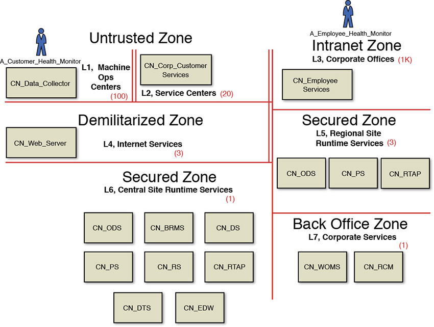
The two primary actors that interact with the Elixir system are as follows:
• A_Customer_Health_Monitor—Corporate customers who access the services of the system.
• A_Employee_Health_Monitor—Corporate employees who access the services of the system.
The following CNs were identified for the Elixir system:
• CN_Data_Collector—A conceptual node that collects data from the field operations and gets it ready to be dispatched to the regional or central sites.
• CN_Corp_Customer_Services—A conceptual node that allows corporate customers to interact and browse through the system’s user interface.
• CN_Employee_Services—A conceptual node that allows corporate employees to interact and browse through the system’s user interface.
• CN_Web_Server—A conceptual node that intercepts all of the user’s requests and routes them to the appropriate presentation layer components of the system. Sitting in the DMZ, this node is the only one that has a public-facing IP address.
• CN_ODS—A conceptual node that represents the operational data store. There is one instance of this node in each of the regional sites and in the central site.
• CN_PS—A conceptual node that hosts the presentation layer components of the system. There is one instance of this node in each of the regional sites and in the central site.
• CN_RTAP—A conceptual node that performs the real-time processing of the incoming data and generates the KPIs. There is one instance of this node in each of the regional sites and in the central site.
• CN_EDW—A conceptual node that hosts the data warehouse and data marts required to support the various reporting needs of the system. There is only one instance of this node, and it resides in the central site.
• CN_DTS—A conceptual node that performs the data exchange between the CN_ODS nodes and the CN_EDW node.
• CN_RS—A conceptual node that hosts and supports the various reporting needs of the system. There is only one instance of this node residing in the central site and that caters to all the reporting needs across both the central site as well as all the regional sites.
• CN_BRMS—A conceptual node that hosts the various components of the business rules engine. There is only one instance of this node, and it resides in the central site and caters to all the business rules needs across both the central site as well as all the regional sites.
• CN_DS—A conceptual node that stores all the user details and its associated authentication and authorization credentials.
• CN_WOMS—A conceptual node that hosts the corporate’s work order management system.
• CN_RCM—A conceptual node that hosts the corporate’s reliability-centered maintenance system.
If you referred back to Chapter 5, specifically to Figure 5.5, which depicted the enterprise view of Elixir, you likely noticed the three enterprise applications—PES System, CAD System, and the Enterprise HRMS System—in addition to other ABBs. The COM model, however, does not have any CNs representing these three systems. CAD and Enterprise HRMS are out of scope of the first release of Elixir and hence are not represented. For the PES System, the data would be transferred to the Engineering Data Warehouse; that is, CN_EDW. It was also decided that the IT department of BWM, Inc., would handle the transfer of the required data by leveraging some data integration techniques (see the “Case Study: Integration View of Elixir” section in Chapter 9, “Integration: Approaches and Patterns”). This data transfer is transparent to the rest of the system, and to keep the architecture as simple as possible, these two systems were not depicted. However, it is entirely appropriate to depict them, if so desired. I chose to keep things simple.
Figure 8.15 represents the various PDUs, DDUs, and EDUs of the Elixir system. The deployable units are represented in italics. A brief description of the deployable units is as follows, arranged by the DU categories.
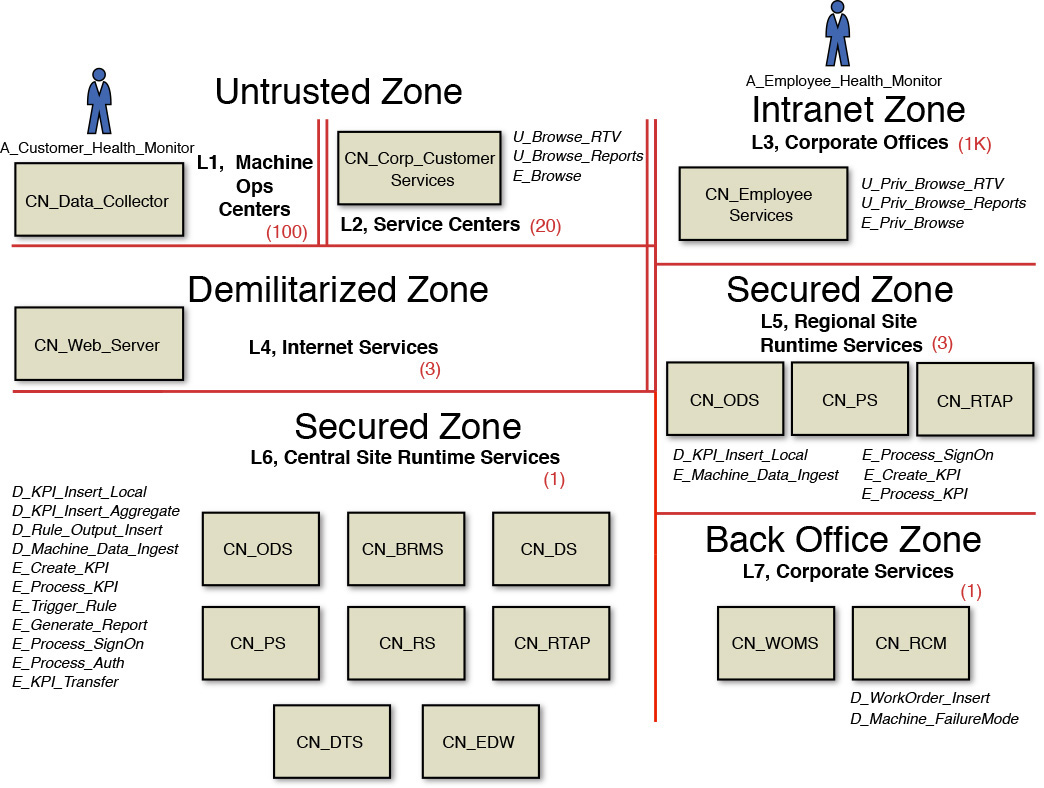
The PDUs are as follows:
• U_Browse_RTV—A PDU that allows corporate customers access to the real-time visualization interfaces.
• U_Browse_Reports—A PDU that allows corporate customers access to the suite of business intelligence reports and their visual user interfaces.
• U_Priv_Browse_RTV—A PDU that allows corporate employees access to the real-time visualization interfaces.
• U_Priv_Browse_Report—A PDU that allows corporate employees access to the suite of business intelligence reports and their visual user interfaces.
• D_KPI_Insert_Local—A DDU that represents the KPI data entity generated by the CN_RTAP node.
• D_KPI_Insert_Aggregate—A DDU that represents rolled-up KPI values aggregated to each cycle of machine operations. This entity is persisted in the CN_EDW node.
• D_Rule_Output_Insert—A DDU that represents the data entity encapsulating the outcome of triggered business rules executed on the CN_BRMS node.
• D_Machine_Data_Ingest—A DDU that encapsulates a message packet that enters the CN_RTAP node.
• D_WorkOrder_Insert—A DDU that represents a work order item that gets created in the CN_WOMS node.
• D_Machine_FailureMode—A DDU that represents an entity that gets retrieved from the CN_RCM node.
The EDUs are as follows:
• E_Browse—An EDU that is capacity sized to host the PDUs in the service centers.
• E_Priv_Browse—An EDU that is capacity sized to host the PDUs in the corporate offices.
• E_Create_KPI—An EDU that is capacity sized to meet the service-level requirements of the CN_ODS node.
• E_Process_KPI—An EDU that is capacity sized to meet the service-level requirements of the CN_RTAP node.
• E_Trigger_Rule—An EDU that is capacity sized to meet the service-level requirements of the CN_BRMS node.
• E_Generate_Report—An EDU that is capacity sized to meet the service-level requirements of the CN_RS node.
• E_Process_SignOn—An EDU that is capacity sized to meet the service-level requirements of the CN_PS node.
• E_Process_Auth—An EDU that is capacity sized to meet the service-level requirements of the CN_DS node.
• E_KPI_Transfer—An EDU that is capacity sized to meet the service-level requirements of the CN_DTS node.
Note that no EDUs are identified for the nodes in the Back Office Zone. The reason is that the nodes in this zone already exist as a part of the corporate IT landscape, and hence, no further definition and design for its placement and capacity sizing are required. Again, I tried to keep things as simple as possible—a mantra that I can chant as long as it may take for it to become imprinted into your architect DNA!
SOM
The SOM for the Elixir system is a set of specification-level nodes that are distributed across the various zones of the OM. Figure 8.16 presents the SOM.
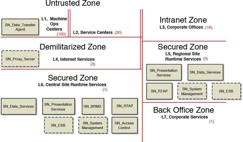
The rest of the section provides a brief description of each of the SOM nodes.
• SN_Data_Transfer Agent—A specification-level node that hosts the CN_Data_Collector conceptual node.
• SN_Proxy_Server—A specification node, implemented as a technical component, that intercepts user requests and applies load balancing and security checks among other things such as caching and compression, before granting access to the requested application functionality.
• SN_Data_Services—A specification node that hosts the data storage and data transfer–related components. It is expected to have two different capacity models. The first capacity model is to support hosting the CN_DTS, CN_EDW, and the CN_ODS conceptual nodes in the Central Site Runtime Services zone. The second capacity model is to support hosting only the CN_ODS conceptual node for each of the Regional Site Runtime Services zones.
• SN_Presentation_Services—A specification node that hosts the CN_PS conceptual node.
• SN_BRMS—A specification node that hosts the CN_BRMS conceptual node.
• SN_RTAP—A specification node that hosts the CN_RTAP conceptual node.
• SN_Systems_Management—A specification node, implemented as a technical component, supporting the systems monitoring and management needs for all the components in a given location. This component supports two different capacity models, one each for the Central Site Runtime Services and the Regional Site Runtime Services, respectively.
• SN_Access_Control—A specification node, implemented as a technical component, that enables user authentication and authorization along with the application of any required security management runtime policies.
• SN_ESB—A specification node, implemented as a technical component, that supports high-speed, low-latency, asynchronous data transfer between the Regional Site Runtime Services and the Central Site Runtime Services locations. The technical component is also capable of supporting mediation, transformation, and routing needs for heterogeneous data sets, message, and transfer protocols.
It is important to note that some of the technical components—for example, SN_BRMS, SN_RTAP, and SN_ESB—are enterprise-level components and hence may be leveraged in multiple enterprise systems (that is, not just for Elixir). Note also, that I have skipped the walkthrough diagrams here; suffice it to say that such due diligence is mandatory as a part of the SOM definition activity.
POM
The POM for the Elixir system is also developed and is represented in Figure 8.17.
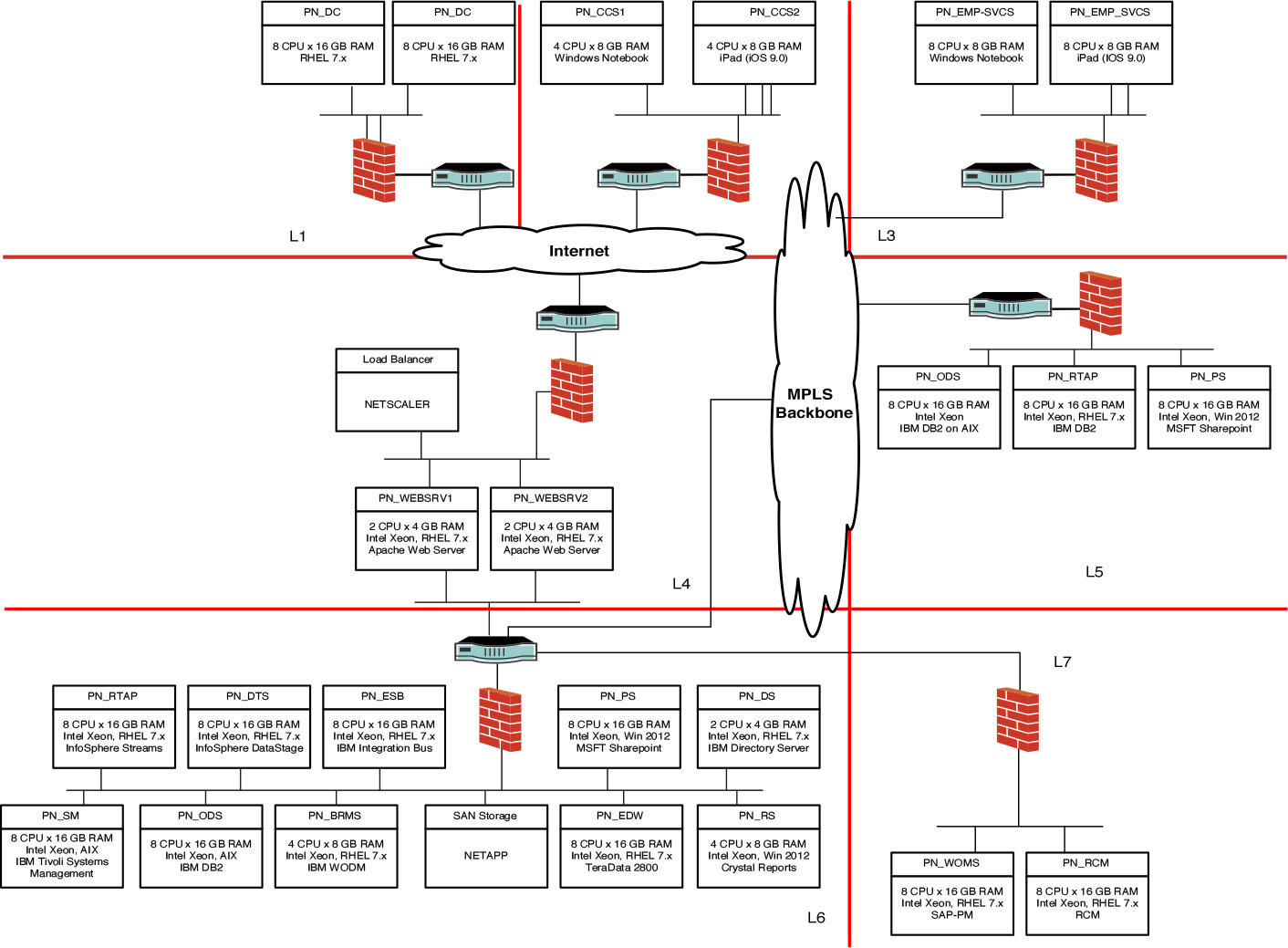
It is important to realize that the POM is developed by simulating a real-world customer scenario; the customer had a set of existing technologies that were leveraged—primarily Teradata (for CN_EDW) and Microsoft SharePoint (for CN_PS). Also, the bias toward IBM’s analytic capabilities influenced the choice of the IBM technologies. Your solution architecture’s POM may well be quite different; in fact, it may not even resemble anything quite like that of Elixir. I presented the POM in this case study as a guideline to drive the design and formulation of the POMs you will forever innovate!
Summary
Operational modeling is one of the foundational domains of software architecture focusing on addressing the nonfunctional aspects of the system. It is by no means a trivial subdiscipline of solution architecture. The operational model is iteratively developed through three major phases: the conceptual operational model (COM), the specification operational model (SOM), and the physical operational model (POM). The COM provides a technology-neutral view of the operational model focusing primarily on the application-level components. The SOM turns its attention to the service-level requirements. It not only introduces the executable compute nodes on which the application-level components would run but also identifies a set of technical components that support the system’s interconnects, integration needs, systems management, and monitoring needs, along with their required network support. The technical components are identified and their specifications are defined to support the business functions along with their appropriate service-level agreements. The POM provides a blueprint for the procurement, installation, and subsequent monitoring and maintenance of the system. It consolidates the hardware infrastructure along with the physical servers required for the fully operational system.
It is quite natural and realistic to develop the OM through partial parallelism of the phases. The SOM can be split into two iterations. The first iteration may focus on the application-level components, while the second iteration may focus on the technical-level components that are required to support the application components, thereby ensuring that they support the required characteristics. The POM too can be split into two iterative developments. The first iteration may focus on the component selection; that is, identifying the technologies and products that will be used to build the various parts of the OM. The second iteration can, later on, focus on how the technologies will be put together and configured to deliver to the final specifications. It is quite common to perform the first iteration of the POM in parallel with the SOM iterations.
Much like the discussion in the previous chapter about the time-critical nature of almost all IT projects, it is very important to identify every opportunity to parallelize the activities in the various phases of the OM development. Prior knowledge of the system, the IT landscape, the architectural blueprint, the vendor selection policies, and personal or organizational bias must be understood, acknowledged, and appropriately leveraged. Cost and time constraints may push you to start with the SOM and then work your way to a final POM. In such a scenario, here is some advice: you can leverage the first of the two SOM iterations as your virtual COM. In such time-constrained scenarios, my only suggestion would be to add a little bit more time to the SOM phase and tell your project manager that you got rid of the entire COM phase!
As a parting note from this chapter, I strongly recommend that the solution architect in you should mandate that a well-experienced infrastructure architect must be working with you to formalize the OM. Do not shy away from using the help of a network architect either; I call the infrastructure and network architect roles the specialist architects. And although we have not touched upon other areas (for example, security and testing), security architects and test architects also fall under the category of specialist architects. And if you have come this far, you should know enough to be able to engage with your specialist architects—that is, to be able to guide them to build the OM.
The Elixir case study now has an operational model.
Take a step back, relax, take a deep breath, and appreciate the various frontiers of solution architecture that you have mastered so far!
References
“Deployment Operational Models.” (n.d.). Retrieved from http://dodcio.defense.gov/Portals/0/Documents/DODAF/Vol_1_Sect_7-2-2_Deployment-Operational_Models.pdf