
CHAPTER 4
PROBABILITY AND TEXT SAMPLING
Chapters 2 and 3 introduce and explain many features of Perl. Starting at this point, however, the focus shifts to using it for text analyses. Where new features are introduced, these are noted and explained, but the emphasis is on the texts.
This chapter focuses on some of the statistical properties of text. Unfortunately, some of the common assumptions used in popular statistical techniques are not applicable, so care is needed. This situation is not surprising because language is more complex than, for example, flipping a coin.
We start off with an introduction to the basics of probability. This discussion focuses on the practical, not the theoretical, and all the examples except the first involve text, keeping in the spirit of this book.
Probability models variability. If a process is repeated, and if the results are not all the same, then a probabilistic approach can be useful. For example, all gambling games have some element of unpredictability, although the amount of this varies. For example, flipping a fair coin once is completely unpredictable. However, when flipping a hundred coins, there is a 95% probability that the percentage of heads is between 40% and 60%.
Language has both structure and variability. For example, in this chapter, what word appears last, just before the start of the exercises? Although some words are more likely than others, and given all the text up to this point, it is still impossible to deduce this with confidence.
Even guessing the next word in a sequence can be difficult. For example, there are many ways to finish sentence 4.1.
(4.1) Crazed by lack of sleep, Blanche lunged at me and screamed “...."
Because language is so complex, coin flipping is our first example, which introduces the basic concepts. Then with this in mind, we return to analyzing English prose.
4.2.1 Probability and Coin Flipping
First, we define some terms. A process produces outcomes, which are completely specified. How these arise need not be well understood, which is the case for humans producing a text. However, ambiguous outcomes are not allowed. For example, a person typing produces an identifiable sequence of characters, but someone writing longhand can create unreadable output, which is not a process in the above sense.
For processes, certain groups of outcomes are of interest, which are called events. For example, if a coin is flipped five times, getting exactly one head is an event, and this consists of the five outcomes HTTTT, THTTT, TTHTT, TTTHT, and TTTTH, where H stands for heads and T for tails. Notice that each of these sequences completely specifies the result of the process.
The probability of an event is a number that is greater than or equal to zero and less than or equal to one. For a simple process, probabilities can be computed exactly. For example, the probability of exactly one head in five flips of a fair coin is 5/32. However, because language is complex and ever changing, probabilities for text events are always approximate, and our interest is in computing empirical probabilities, which are estimates based on data.
For the first example, we estimate the empirical probability of heads from the results of computer-simulated coin flips. The simplest method for doing this is to count the number of events and divide by the number of results. Let n () be the function that returns the number of times its argument occurs, then equation 4.2 summarizes the above description.
(4.2) ![]()
We use this equation to estimate the probability of getting a head. Perl has a function called rand that returns a random number between 0 and 1. This can generate coin flips as follows: if rand is greater than 0.5, then the result is H, else it is T. Note that rand is not truly random (such computer functions are called pseudorandom), but we assume that it is close enough for our purposes. Using this idea, the following command line argument runs program 4.1 to simulate 50 flips.
perl flip.pl 50
The argument after the program name (50 in the above example) is stored in $ARGV [0], which determines the number of iterations of the for loop. When this is finished, the empirical probability estimate of getting a head is computed.
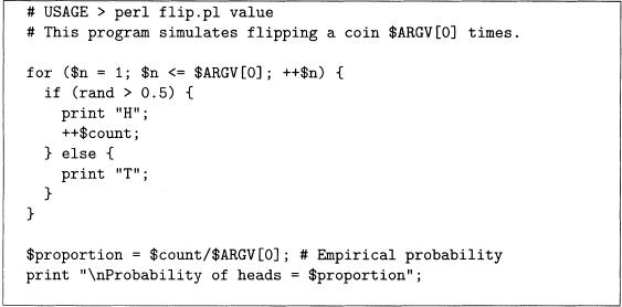
Program 4.1 This program simulates coin flips to estimate the probability of heads.
Output 4.1 shows one run of program 4.1 that produces 23 heads out of 50 flips, which is 46%. By equation 4.2, this proportion is the empirical probability estimate of getting a head. Clearly running this program a second time is likely to give a different estimate, so this estimate is an approximation.
Output 4.1 Output of program 4.1 for 50 flips.
HTHHHHHHHTHHHTTTTHTHTHTTTTHHTTTHTTHTHTTTHTTHTTTHHT |
Probability of heads = 0.46 |
Because it is well known that the probability of heads is 0.5, program 4.1 might seem like a waste of time. But keep in mind two points. First, to estimate the probability of the word the occurring in some text, there is no theoretical solution, so we must use an empirical estimate. Second, even for coin tossing, there are events that are hard to compute from theory, and the empirical answer is useful either for an estimate or a check of the true probability. See problems 4.1 and 4.2 for two examples of this.
In addition, the above output can be used to estimate the probability of heads after the first flip, after the second flip, and so forth, until the last flip. If empirical estimates are useful, then as the number of flips increases, the probability estimates should get closer and closer to 0.5 (on average). Although this is tedious to do by hand, it is straightforward to modify program 4.1 to print out a running estimate of the probability of heads. This is done with the variable $proportion inside the for loop of program 4.2.
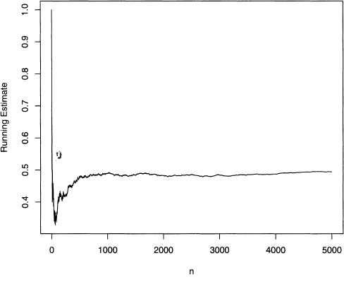
This program produces the running probability estimates shown in figure 4.1. Note that near the end of the 50 flips the estimates gets worse. Large deviations are always possible, but they are more and more unlikely as the number of flips increases. Finally, figure 4.2 shows an example of 5000 flips. Here the initial large deviations die out as the number of flips gets larger.
Figure 4.1 Plot of the running estimate of the probability of heads for 50 flips.
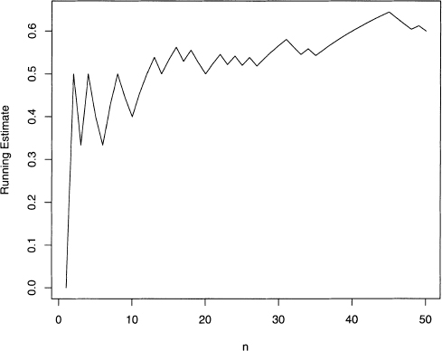
Figure 4.2 Plot of the running estimate of the probability of heads for 5000 flips.
Although coins can be flipped more and more, samples of text have an upper limit. For example, Edgar Allan Poe is dead, and any new works are due to discovering previously unknown manuscripts, which is rare. Hence, it is often true with texts that either the sample cannot be made larger, or it is labor intensive to increase its size. Unfortunately, there are measures of a text that do not converge to a fixed value as the sample size increases to its maximum possible value (see section 4.6). Hence working with texts is trickier than working with simpler random processes like coins.
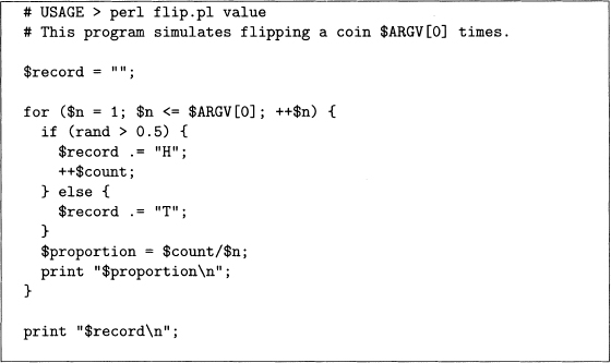
Program 4.2 Modification of program 4.1 that produces arunning estimate oftheprobability of heads.
4.2.2 Probabilities and Texts
Consider this problem: find an estimate of the probability of each letter of the alphabet in English. For a fair coin, assuming the probabilities of heads and tails are equal is reasonable, but for letters this is not true. For example, the letter a is generally more common than the letter z. Quantifying this difference takes effort, but anyone fluent in English knows it.
To estimate letter frequencies, taking a sample of text and computing the proportion of each letter is a reasonable way to estimate these probabilities. However, a text sample that is too short can give poor results. For example, sentence 4.3 gives poor estimates.
(4.3) Ed’s jazz dazzles with its pizazz.
Here z is the most common letter in this sentence comprising 7 out of the 27, or a proportion of almost 26%. Obviously, most texts do not have z occurring this frequently.
There is an important difference between the coin example in the last section and this example. In output 4.1, an estimate of 46% for the probability of heads is found by flipping a coin 50 times, which is close to the correct answer of 50%. However, there are 26 letters in the alphabet (ignoring case and all other characters), and letters are not used equally often. Such a situation requires larger sample sizes than coin flipping.
Note that sentence 4.3 has no bs, which is a proportion of 0%, but all the letters of the alphabet have a nonzero probability, so this estimate is too low. This reasoning is true for all the letters that do not appear in this sentence. Moreover, the existence of estimates that are too low imply that one or more of the estimated probabilities for the letters that do appear are too high. Having estimates that are known to be either too high or too low is called bias. The existence of zero counts produces biased probability estimates, and, to a lesser degree, so do very low counts.
Hence using proportions from samples as estimates of probabilities requires sample sizes that are large enough. Quantifying this depends on the size of the probabilities to be estimated, but if there are possible events that do not appear in the sample, then a larger sample is useful. However, as noted above, a larger example may not be possible with text.
Finally, coin flipping is not immune to the problem of bias. For instance, if we flip the coin only one time, the empirical probability of heads is either 0 or 1, and both of these answers are the furthest possible from 0.5. However, additional flips are easy to obtain, especially if a computer simulation is used. With the above discussion in mind, we estimate letter probabilities.
4.2.2.1 Estimating Letter Probabilities for Poe and Dickens As noted in the last section, using sentence 4.3 to estimate the probability of each letter gives misleading results. However, a larger text sample should do better. Because counting letters by hand is tedious, this calls for Perl. It is easy to break a string into characters by using the function split with the empty regular expression as its first argument (empty meaning having no characters at all). Keeping track of the character counts is done by using the hash %freq (see section 3.6 to review hashes).
To try out program 4.3, we first analyze Poe’s “The Black Cat" [88] using the following command line statement.
pen count_characters .pl The_Black_Cat .txt
The output has two parts. First, all of the characters in the story are listed from most frequent to least frequent. Second, the frequencies of the letters a through z are listed in that order. It turns out that the blank is the most frequent (where newline characters within paragraphs are counted as blanks), with a frequency of 4068. The most frequent letter is e (appearing 2204 times), and the least frequent is z (6 times), which is out of a total of 17,103 letters. Hence, e appears almost 13% of the time, while z appears only 0.035% of the time.
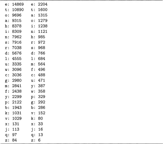
The story “The Black Cat" is only a few pages long, so let us also try a longer work, Charles Dickens’s A Christmas Carol, which can be done by replacing The Black Cat .txt with A_Christmas_Carol.txt in the open statement. Output 4.2 ranks the letters with respect to frequency for both these works of fiction. Although the orders do not match exactly, they are similar. For example, the letter e appears 2204/17, 103 ≈ 12.89% of the time in “The Black Cat," as compared to 14, 869/12 1, 179 ≈ 12.27% for A Christmas Carol. Both of these are close to the value of 13% cited in Sinkov’s Elementary Cryptanalysis [110], which is based on a larger text sample. These similarities suggest that these two works are representative of English prose with respect to letter frequencies.
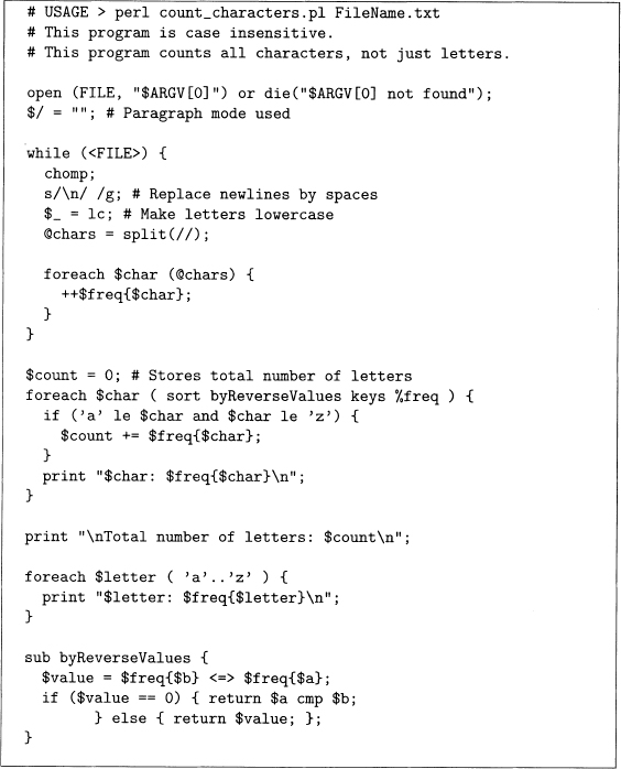
Program 4.3 This program counts the frequency of each character in a text file.
This question of representativeness is key. In sampling, the researcher hopes that the sample is similar to the population from which it is taken, but he or she can always get unlucky. For example, Georges Perec wrote the novel La Disparition without using the letter e, which is the most common letter in French (and English). This novel was translated by Gilbert Adair into English with the title A Void [87]. He was faithful to the original in that he also did not use the letter e. So if we pick the English version of this novel, the estimate of the probability of the letter e is 0%, which is clearly anomalous. However, A Void is not a representative sample of English prose. This kind of a literary work (one that does not use a specific letter) is called a lipograin.
Output 4.2 Output of program 4.3 for both Dickens’s A Christmas Carol and Poe’s “The Black Cat”. Letters are listed in decreasing frequency.
Finally, output 4.2 shows that both stories use all the letters of the alphabet. Unfortunately, for more complex sets of strings that are of interest to linguistics, usually some are not represented in any given sample. For example, the next section shows that counting letter pairs produces many zero counts. As noted at the start of this section, these are underestimates, which makes at least some of the nonzero counts overestimates, both of which cause biases in the probability estimates.
4.2.22 Estimating Letter Bigram Probabilities From single letters, the next step up in string complexity are pairs, which are called letter bigrams. These are ordered pairs, that is, the order of the letters matters. For example, the title “The Black Cat” has the following letter bigrams: th, he, bl, la, ac, ck, ca, and at. Here both case and the spaces between the words are ignored. Depending on the application, however, treating a space as a character can be useful. Also, a decision on whether to keep or to ignore punctuation is needed. For this section, nonletter characters are deleted, except for hyphenated words. In this case, the hyphens are replaced with spaces, for example, self-evident is split into self and evident.
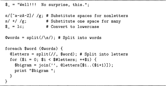
To do this, first, substitute all nonletters with spaces with s/ [ˆa–zA–Z] / /g. Second, change multiple spaces into one space, which is done by another substitution. Third, convert all the letters to lowercase with the lc function. Then convert the text into words with the split function (splitting on whitespace), followed by splitting each word into letters. Finally, the letters are combined into pairs with the join function. All these steps are done in code sample 4.1, which produces output 4.3.
Code Sample 4.1 Code to find letter bigrams contained in the string stored in $-.
Output 4.3 The bigram output of code sample 4.1.
we el 11 no su ur rp pr ri is se th hi is |
Code sample 4.1 works for the test string, so we use it to construct a bigram counting program. The result is program 4.4, which uses byReverseValues from program 4.3.
Program 4.4 produces much more output than program 4.3 since there are 262 = 676 possible bigrams. Applying this to A Christmas Carol produces 415 bigrams, the 10 most frequent are given in output 4.4. Note that 676 – 415 = 261 bigrams that do not appear in this novel.
The fact that many bigrams are missing (a little more than a third) is not surprising. For example, it is difficult to think of a word containing xx or tx. However, such words exist. For example, for a list of 676 words that contains each of the 676 possible bigrams, see section 31 of Making the Alphabet Dance [411 by Eckler. However, words are not the only way these bigrams can appear. For example, XX is the roman numeral for 20 and TX is the postal code for Texas. Moreover, there are many other types of strings besides words that can be in a text. For example, a license plate can easily have one of these two bigrams. Hence, the missing bigrams are possible, so a proportion of 0% is an underestimate.
In general, with even long texts it is not hard to find words or phrases that are not unusual yet do not appear in the text. For example, of the days of the week, Tuesday, Wednesday, and Thursday do not appear in A Christmas Carol (although Friday does appear, it refers to the character with that name in Robert Louis Stevenson’s Treasure Island.) Unfortunately, this means the problem of having proportions that are 0% is generally unavoidable when working with texts.
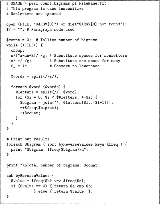
Program 4.4 This program counts the frequency of each bigram in the text file specified on the command line.
Output 4.4 The 10 most frequent bigrams found by program 4.4 for Dickens’s A Christma Carol.
th: | 3627 |
he: | 3518 |
in: | 2152 |
an: | 2012 |
er: | 1860 |
re: | 1664 |
nd: | 1620 |
it: | 1435 |
ha: | 1391 |
ed: | 1388 |
Finally, before moving on, it is not hard to write a Perl program to enumerate letter triplets (or trigrams). See problem 4.4 for a hint on doing this. We now consider two key ideas of probability in the next section: conditional probability and independence.
The idea of conditional probability is easily shown through an example. Consider the following two questions. First, for a randomly picked four-letter word (from a list of English words), what is the probability that the second letter is u? Second, for a randomly picked four-letter word that starts with the letter q, what is the probability that the second letter is u?
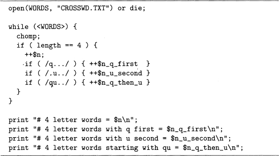
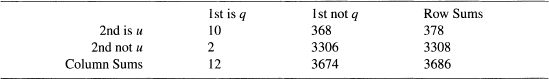
Given a word list and a Pen program, these questions are answerable, and with regular expressions, it is not hard to create such a program. Grady Ward’s Moby Word Lists [123] has the file CROSSWD. TXT, which has more than 110,000 total words, including inflected forms. Code sample 4.2 counts the following: all four-letter words, all four-letter words starting with q, all four-letter words with u as the second letter, and all four-letter words starting with qu. Note that chomp must be in the while loop: try running this code sample without it to see what goes wrong. Finally, the results are given in output 4.5.
Now we can answer the two probability questions. Since there are 3686 four-letter words, and 378 of these have u as their second letter, the probability that a randomly selected four-letter word has u as the second letter is 378/3686, which is close to 10%. But for the second question, only the 12 four-letter words starting with q are considered, and of these, 10 have u as the second letter, so the answer is 10/12, which is close to 83%.
Knowing English, it is no surprise that the most common letter following q is u. In fact, having an answer as low as 83% may be surprising (the two exceptions are qaid and qoph). Because u is typically the least common vowel (true in output 4.2 for “The Black Cat" and A Christmas Carol), it is not surprising that as little as 10% of four-letter words have u in the second position.
Although the above example is a special case, the general idea of estimating conditional probabilities from data does not require any more theory, albeit there is some new notation. However, the notation is simple, widely used, and saves time, so it is worth knowing.
Suppose A is an event. For example, let A stand for obtaining a head when flipping a coin once. Then P(A) is the probability of event A happening, that is, the probability of getting heads. In statistics, the first few capital letters are typically used for events. For example, let B stand for a randomly picked four-letter word with u as its second letter. Then, as discussed above, P(B) = 378/3686, at least for Grady Ward’s CROSSWD. TXT word list.
Code Sample 4.2 An analysis of four-letter words.
Output 4.5 Word counts computed by code sample 4.2.
# 4 letter words = 3686 |
# 4 letter words with q first = 12 |
# 4 letter words with u second = 378 |
# 4 letter words starting with qu = 10 |
In symbols, conditional probability is written P(B|C), which means “the probability of event B happening given that event C has already happened.’ This is usually read as “the probability of B given C." For example, let B be the event defined in the preceding paragraph, and let C be the event that a randomly selected four-letter word has q as its first letter. Then P(B|C) is the probability that the second letter is u given that the first letter of a randomly selected four-letter word is q. As computed above, P(B|C) = 10/12.
The general formula is straightforward. For any two events E and F, P(E|F) assumes that F has, in fact, happened. So the computation requires two steps. First, enumerate all outcomes that comprise event F. Second, of these outcomes, find the proportion that also satisfies event E, which estimates PP(E|F). Equation 4.4 summarizes this verbal description as a formula, where and is used as in logic. That is, both events connected by and must happen.
(4.4) ![]()
For the example of four-letter words discussed above, “B and C" means that both B and C must occur at the same time, which means a four-letter word starting with qu. There are 10 words that satisfy this in the file CROSSWD .TXT (they are quad, quag, quai, quay, quey, quid, quip, quit, quiz, quod). This is out of all the four-letter words starting with q (which also includes qaid and qoph to make a total of 12). Finally, equation 4.4 says P(B|C) is the ratio of these two numbers, so it is 10/12, as claimed above.
Here is one more way to think about conditional probability. Let n be the total number of possibilities. Then equation 4.5 holds.
(4.5) ![]()
Using B and C as defined above, let us check this result. In equation 4.6, note that the number of four-letter words (3686) cancels out to get 10/12.
(4.6) 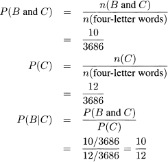
Finally, it is important to realize that order of events matters in conditional probability. That is, P(B|C) is generally different from P(C|B), and this is the case for B and C defined above. For these events, P(C|B) is the probability of a randomly picked fourletter word having q as its first letter given that u is its second letter. Given this, there are many four-letter words that begin with letters other than q, for example, aunt, bull, cups, dull, euro, and full. Hence this probability should be much smaller than 83%, the value of P(B|C). Using output 4.5, it is 10/378, or about 2.6%. Note that this numerator is the same as the one for P(B|C), which is no accident since “B and C" is the same event as “C and B." However, the denominators of P(B|C) and P(C|B) are quite different, which makes these probabilities unequal.
Related to conditional probability is the concept of independence of events, which allows computational simplifications if it holds. With text, however, independence may or may not hold, so it must be checked. This is the topic of the next section.
4.3.1 Independence
Examples of two independent events are easy to give. For instance, as defined above, let A stand for a coin flip resulting in a head, and let B stand for a randomly picked four-letter word that has u as its second letter. Since coin flipping has nothing to do with four-letter words (unless a person has lost large sums of money betting on the coin), knowing that A has occurred should not influence an estimate of the probability of B happening. Symbolically, this means P(B|A) = P(B), and, in fact, this can be used as the definition of independence of A and B. Moreover, since four-letter words do not influence coin flips, it is also true that P(A|B) = P(A).
These two equalities and equation 4.5 imply that equation 4.7 holds when F and F are independent events. This result is called the multiplication rule.
(4.7) 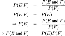
The closer P(E and F) is to P(E)P(F), the more likely it is that E and F are independent. Returning to events B and C of the last section, we can check if these are independent, although intuition of English suggests that q at the beginning of a four-letter word and u in the second position are not independent. That is, they are dependent.
Fortunately, all the needed probabilities are already computed, which are summarized in equation 4.8. The two values are different by a factor of 8.1. Although the precise boundary that distinguishes dependence from independence is not obvious, a factor of 8.1 seems large enough to support the intuition that q and u are dependent. See problem 4.5 for a statistical test that strongly confirms this.
(4.8) 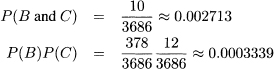
With the ideas of conditional probability and independence introduced, let us consider one more theoretical idea. In text mining, counting is a key step in many analyses. In the next section we consider the ideas of the mean and variance of a numeric measurement.
4.4 MEAN AND VARIANCE OF RANDOM VARIABLES
This section introduces random variables, which are widely used in the statistical literature. These are a convenient way to model random processes.
Random variables are written as uppercase letters, often toward the end of the alphabet, for example, X, Y, or Z. In this book, a random variable is a numeric summary of a sample of text. For example, let X be the number of times the word the appears in a randomly selected text.
Random variables look like algebraic variables and can be used in algebraic formuormulas. However, unlike algebraic equations, we do not solve for the unknown. Instead, think of random variables as random number generators. For text mining, random variables are often counts or percentages, and the randomness comes from picking a text at random.
As a second example, let Y be the proportion of the letter e in a text. Once a text is specified, then Y is computable. For example, in section 4.2.2.1 the letters of A Christmas Carol are tabulated. For this text Y equals 14,869/12 1,179, or about 0.1227. If the Poe short story “The Black Cat" were picked instead, then Y is 2204/17,103, or about 0.1289. Clearly Y depends on the text.
The hope of formulating this problem as a random variable is that as more and more texts are sampled, some pattern of the values becomes clear. One way to discover such a pattern is to make a histogram. For example, if all the values are close together, then an accurate estimate based on this sample is likely.
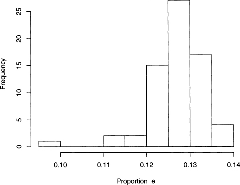
Let us consider the 68 Poe short stories from [96], [97], [98], [99] and [100] with respect to the proportion of the letter e in each one. For some hints on how to do this, see problem 4.6. The results are listed in table 4.1 and then plotted in figure 4.3. This histogram shows a clear peak just below 0.13, and all the values are between 0.11 and 0.14, except for an unusually low one of 0.0989. This comes from “Why the Little Frenchman Wears His Hand in a Sling," which is narrated in a heavy dialect with many nonstandard spellings. Otherwise, Poe is consistent in his use of the letter e.
Table 4.1 Proportions of the letter e for 68 Poe short stories, sorted smallest to largest.
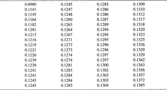
Figure 4.3 Histogram of the proportions of the letter e in 68 Poe short stories based on
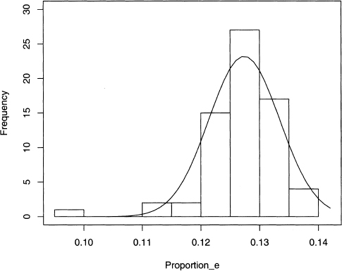
The histogram in figure 4.3 is an empirical approximation of the proportion of e’s in Poe’s short stories. It suggests that a normal distribution is a good model, which is supported by the good fit of the curve drawn in figure 4.4. The mean and standard deviation of this curve are estimated by the respective sample values, which are 0.1274 and 0.0060.
Figure 4.4 Histogram and best fitting normal curve for the proportions of the letter e in 68 Poe short stories.
The standard deviation is one popular measure of variability. In general, to say precisely what it measures depends on the shape of the data. For distributions that are roughly bell-shaped (also called normally distributed), it can be shown that the mean and standard deviation provide an excellent summary of the shape.
Nonetheless, there are constraints and heuristics for this concept. For example, the standard deviation is a number greater than or equal to zero. Zero only occurs if there is no variability at all, which means that all the values in the data set are exactly the same. The larger the standard deviation, the more spread out the values, which makes the histogram wider. To say more than this, we need to know something about the shape of the data. Below we assume that the histogram is approximately bell-shaped.
First, we define some notation. Let the mean value of the data (called the sample mean) be denoted by a bar over the letter used for the associated random variable, or ![]() in this case. Second, let the standard deviation of the data (called the sample standard deviation) be denoted by the letter s with the random variable given as a subscript, for example, Sy. Now we consider the range of values
in this case. Second, let the standard deviation of the data (called the sample standard deviation) be denoted by the letter s with the random variable given as a subscript, for example, Sy. Now we consider the range of values ![]() – Sy to
– Sy to ![]() + Sy. This is an interval centered at
+ Sy. This is an interval centered at ![]() , and its length is 2Sy, a function of only the standard deviation. Assuming bell-shaped data, then about 68% of the values lie in this interval. A more popular interval is
, and its length is 2Sy, a function of only the standard deviation. Assuming bell-shaped data, then about 68% of the values lie in this interval. A more popular interval is ![]() – 2Sy to
– 2Sy to ![]() + 2Sy, which contains about 95% of the data. Note that the length of this is 4Sy, which makes it twice as wide as the first interval.
+ 2Sy, which contains about 95% of the data. Note that the length of this is 4Sy, which makes it twice as wide as the first interval.
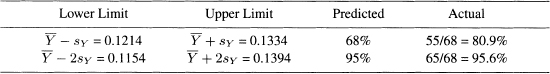
For the Poe stories, Sy is 0.0060 (see equation 7.2 for a formula), and we can construct the two intervals given above, which is done in table 4.2. Note that 55 out of the 68 stories have e proportions in the smaller interval, and this is 80.9%, which is bigger than the predicted 68%. However, the second interval has 65 out of the 68 stories, which is 95.6%, or practically 95%. In general, data that looks roughly bell-shaped need not fit the theoretical normal curve perfectly, yet the predicted percentages are often close to the theoretical ones.
Finally, there are other types of intervals. The next section, for example, considers intervals to estimate the population mean.
4.4.1 Sampling and Error Estimates
One common framework in statistics is taking a sample from a population. The latter is a group of items of interest to the researcher, but measuring all of them is too expensive (either in time or resources or both). Measuring only a subset of these items is one way tc reduce the costs. The smaller the sample, the cheaper the analysis, but also the larger the error in the estimates (on average). So there is always a trade-off between accuracy and cost in sampling.
Numerical properties of the population are called parameters. These can be estimated by constructing a list of the population and then selecting a random subset from this list. For this discussion, a random sample is a method of picking items so that every item has the same probability of selection, which is called a simple random sample. There are, however, many types of samples: see section 6.2.1 for an example.
Now reconsider the proportion of the letter e data from the last section. Suppose we believe that Poe’s use of this letter is not something he tried to purposely manipulate. Then it is plausible that Poe has a typical proportion of its use. This value is an unknown parameter, and we want to estimate it by taking a sample of his works and computing its average. Since different stories use different words, the percentage of e in each work varies, and so an estimate of the standard deviation is also of interest. Again this is an unknown parameter of Poe, so we estimate it by computing the standard deviation of the sample. If the data in the sample is roughly bell-shaped, then the mean and the standard deviation is a good summary of the data. For more on what is meant by this, see problem 4.7.
For conciseness, let us introduce these symbols. First, let the unknown population mean be μp where the p stands for Poe. This is estimated by computing the sample mean ![]() . Second, let the unknown population standard deviation be σp. This is estimated by the sample standard deviation, Sy.
. Second, let the unknown population standard deviation be σp. This is estimated by the sample standard deviation, Sy.
If we believe our data model that the sample has a bell-shaped histogram, which is visually plausible in figure 4.4, then not only can μp be estimated, but its error is estimable, too. One way of doing this is to give an interval estimate of μp along with an estimate of the probability this interval contains μp For example, equation 4.9 gives a 95% confidence interval for the population mean. That is, constructing such an interval successfully contains the true population mean 95% of the time, on average.
(4.9) ![]()
Using the sample mean and standard deviation of the Poe stories, this formula produces the interval 0.1259 to 0.1289. Notice that this is much smaller than the ones in table 4.2. This happens because predicting the mean of a population is more precise than predicting an individual value for a sample size of 68.
Another way to view this equation is that ![]() is the best estimate of the population mean, and that 2sy/
is the best estimate of the population mean, and that 2sy/![]() is an error estimate of
is an error estimate of ![]() . For more information on a variety of confidence intervals, see Statistical Intervals: A Guide for Practitioners by Hahn and Meeker [49].
. For more information on a variety of confidence intervals, see Statistical Intervals: A Guide for Practitioners by Hahn and Meeker [49].
Finally, we consider the randomness of the selection of the 68 Poe short stories used above, which are obtained from a public domain edition available on the Web. First, some of these are not short stories, for example, “Maelzel’s Chess Player" [91] is an analysis of a touring mechanical device that was claimed to play chess (and Poe concludes correctly that it hid a human chess player). Second, not all of Poe’s short stories are included in these five volumes, for example, “The Literary Life of Thingum Bob, Esq." is missing. However, most of them are represented. Third, Poe wrote many short pieces of nonfiction, for example, book reviews and opinion pieces. In fact, one of these is included, “The Philosophy of Furniture," in which he discusses his ideas on interior design. Hence, these 68 works are closer to the complete population of his short stories than to a random sample of these.
There is one more complication to consider. If Poe is thought of as a generator of short stories, then these 68 are just a subset of his potential short stories. With this point of view, the population is not clear. In addition, the idea that his existing stories are a random sample of this population is unlikely. For example, he might have written the stories he thought would sell better. Note that in either of these points of view, the stories analyzed are not a random sample of some population. For more on text sampling, see section 6.2.2.
Next we switch from letters to words in a text. Words can be studied themselves or as the building blocks of linguistic objects like sentences. The next section introduces an important, but limited, probability model for words.
4.5 THE BAG-OF-WORDS MODEL FOR POE’S “THE BLACK CAT”
In the next chapter the bag-of-words model is used. In this section we define it and discuss some of its limitations. However, in spite of these, it is still useful.
Analyzing a text by only analyzing word frequencies is essentially the bag-of-words model. Because any random permutation of the text produces the same frequencies as the original version, word order is irrelevant. Note that cutting out each word of a paper version of the text, putting them into a bag, and then picking these out one by one produces a random order. So the term bag-of-words is an appropriate metaphor.
Since the bag-of-words model completely ignores word order, it clearly loses important information. For example, using Perl it is not hard to randomize the words of a text. Output 4.6 contains the first few lines of a random permutation of “The Black Cat" by Poe. For a hint on how to do this, see problem 4.8.
Output 4.6 The first few lines of the short story “The Black Cat” after its words have been randomized and converted to lowercase.
hideous me at above this breast something fell impression had |
the as between down a i body scream caresses the the on and |
put night make or of has ascended been brute into similar blood |
and bosom hit but from entire destroying and search evidence |
frequent to could had and i they why investigation dislodged |
and rid day inquiries from the time the steadily to oh me be |
i and chimney the the old violence graven dared blow understand |
was for appeared in i and of at feelings of took stood aimed hot |
i the concealment of period trouble assassination the for better |
off evident a him this shriek and nook immortal it easily wish |
Although output 4.6 is ungrammatical, itdoes preserve some of Poe’s writing style. For example, it is appropriate (though accidental) that it starts off with hideous me. And it does include many words with negative connotations: hideous, scream, brute, blood, destroying, and so forth. On the other hand, reading the original story is much more enjoyable.
An example of a word frequency text analysis is done in section 3.7.1, which illustrates Zipf’s law applying program 3.3 to Dickens’s novel A Christmas Carol. This program produces the counts needed to create figure 3.1.
Zipf’s law implies words that appear once are the most common, which suggests that authors do not use all the words they know in a text (empirical evidence of this is given in the next section). Hence a text has many zero counts for words known by the author. As noted in section 4.2.2, this implies that these word frequencies have biases. This is an important conclusion, and one based on a bag-of-words model, which shows that a simplistic language model can produce interesting results.
Finally, to finish this chapter, we analyze how word frequencies depend on the size of the text used. This reveals an important difference between coin tossing and texts. Unfortunately, this difference makes the latter harder to analyze.
Section 4.2.1 shows an example of estimating the probability of getting heads by simulating coin flips. Although the results are not exact, as the number of flips increases, the accuracy of the estimate increases on average, as shown by figures 4.1 and 4.2. In this simulation, all the bigger deviations from 0.5 occur below 1000 flips. For coins, the exact answer is known, so an estimate based on simulation is easily checked. However, with a text sample, the exact answer is unknown, and so using samples to make estimates is the only way to proceed.
In the next section, we examine how the number of types is related to the number of tokens as the sample size increases. The texts used are Poe’s “The Unparalleled Adventures of One Hans Pfaall" [95] and “The Black Cat" [88]. We find out below that coins are better behaved than texts. Finally, this example uses the approach described in section 1.1 of Harald Baayen’s book Word Frequency Distributions [6], which analyzes Lewis Carroll’s Alice in Wonderland and Through the Looking Glass. If word frequencies interest the reader, then read Baayen for an in-depth discussion of modeling them.
4.6.1 Tokens vs. Types in Poe’s “Hans PfaaII"
In section 3.1, a distinction is made between tokens and types, which we now apply to words. First, as tokens, every word is counted, including repetitions. Second, as types, repetitions are ignored. Recall sentence 3.1: The cat ate the bird. It has five tokens, but only four types.
In this section we show that the number of types is a function of the number of tokens, which is the length of a text sample. Because some words are very common (for example, prepositions and pronouns), the number of tokens is generally much greater than the number of types. We consider just how much greater this is as a function of text size.
First, let us define some notation, which is almost the same as Baayen’s [6] except that his Greek omega is changed to a w here. Let N be the size of the text sample, which is the number of tokens. Suppose the words of a text are known, say by using code similar to program 3.3. Label these words w1, w2, w3, ... Although the order used here is not specified, for any particular example, it is determined by how the program works. Let V(N) be the number of types in a text of size N. Let f(wi, N) be the frequency of word wi in a text of size N. Finally, define the proportion of word wi in a text of size N by equation 4.10.
(4.10) ![]()
Now that the notation is given, let us consider the concrete example of Poe’s “The Unparalleled Adventures of One Hans Pfaall” [95], which is one of his longer short stories. To create samples of varying sizes, we select the first N words for a sequence of values. Then the results can be plotted as a function of N.
First, consider V(N) as a function of N. Since there are only a finite number of types for an author to use, if the sample size were big enough, V(N) should flatten out, which means that no new vocabulary is introduced. In practice, an author can coin new words or create new names (of characters, of locations, of objects, and so forth), so even for an enormous sample, V(N) can keep increasing to the end. But the hope is that this rate of increase eventually becomes small. Mathematically speaking, this means that the slope decreases to near zero.
Programming this in Perl is straightforward. First, convert the text to lowercase, then remove the punctuation. Use split to break lines into words. The number of tokens is just the number of words, which can be used as hash keys. Then the size of the hash is the number of types at any given point. These ideas are implemented in program 4.5.
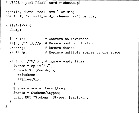
Program4.5 This program computes the ratio of tokens to types for Poe’s “The Unparalleled Adventures of One Hans Pfaall."
In this program, the size of the hash %freq is stored in $types as follows. The function keys returns the keys as an array. Then function scalar forces this array into a scalar context, but this is just the size of the array, which is the number of types in the text. So the combination scalar keys returns the size of the hash. Finally, the results are stored in a comma-separated variable file calledPfaall_word_richness . csv, which then can be imported to a statistical package for plotting (R is used in this book).
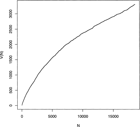
Figure 4.5 is the resulting plot, which clearly shows that V(N) steadily increases as N increases, even at the end of the story. Although the rate of increase is slowing, it is never close to converging to some value. In fact, in the last thousand or so words the slope increases a little, so the limiting value of V(N) is not yet reached. This suggests that Poe’s vocabulary is much bigger than the vocabulary that is contained in this story.
Figure 4.5 Plot of the number of types versus the number of tokens for “The Unparallelec Adventures of One Hans Pfaall." Data is from program 4.5. Figure adapted from figure 1.1 of Baayen [6] with kind permission from Springer Science and Business Media and th author.
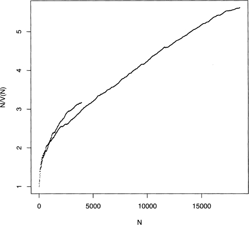
Since V(N) is an increasing function of N, we should take into account the sample size. For example, for coin tossing, the number of heads steadily increases as the number of flips increases, but the proportion of heads stabilizes around 0.5. This suggests that it might be useful to form a ratio of V(N) with N. In section 1.1 of [6], Baayen suggests using the mean word frequency, N/V(N), which is the mean number of tokens per type Program 4.5 already computes this, and the results are plotted in figure 4.6.
Figure 4.6 Plot of the mean word frequency against the number of tokens for “The Unparalleled Adventures of One Hans Pfaall.” Data is from program 4.5. Figure adapted from figure 1.1 of Baayen [6] with kind permission from Springer Science and Business Media and the author.

Unfortunately, this second plot does not flatten out either. In fact, the rate of increasc (or slope) of the plot for N in the range of 3000 to 17,000 is close to constant. Although at the highest values of N the slope of the plot decreases somewhat, it is not clear that it i close to reaching a plateau.
This lack of convergence might be due to the small sample size. After all, this texi is not even 20,000 words long, and perhaps longer texts behave as we expect. However section 1.1 of Baayen [6] states that even for text samples on the order of tens of milliom of words, the mean word frequency still does not converge to a fixed value.
This has practical consequences. Suppose we want to compare “The Black Cat" and “The Unparalleled Adventures of One Hans Pfaall" with respect to vocabulary diversity The stories have different lengths, and it is tempting to believe that this can be taken into account by computing the mean word frequency for both stories. The results seem quite significant: “The Black Cat" has an average of 3.17 tokens per type, while “Hans Pfaall" has a value of 5.61, which is about 75% higher.
However, the mean word frequency depends on sample size. So if we plot N/V(N) vs. N for both stories on the same plot, then we can make a fairer comparison. Program 4.5 is easily modified to count up the number of tokens and types for “The Black Cat.” Once this is done, the plots for both stories are put into figure 4.7 for comparison.
This figure shows that “The Black Cat” has the slightly higher mean word frequency
when we compare both stories over the range of 1000 to 4000 (the latter is approximately the length of “The Black Cat”). Hence the initial comparison of 3.17 to 5.61 tokens per type is mistaken due to the effect of text length. Note that this approach compares the shorter story to the initial part of the longer story, so the two texts are not treated in a symmetric manner.
Figure 4.7 Plot of the mean word frequency against the number of tokens for “The Unparalleled Adventures of One Hans Pfaall” and “The Black Cat.” Figure adapted from figure 1.1 of Baayen [6] with kind permission from Springer Science and Business Media and the author.
In corpus linguistics, researchers typically take samples of equal size from a collection of texts. This size is smaller than each text, so that all of them are analyzed in a similar fashion. The corpora built by linguists use this approach. For example, the Brown Corpus uses samples of about 2000 words. For more information on the construction of this corpus, see the Brown Corpus Manual [46].
This chapter introduces the basics of probability using text examples. These ideas occur again and again in the rest of this book since counting and computing proportions of strings or linguistic items is often useful by itself and is a common first step for more sophisticated statistical techniques.
To learn more about statistics with an exposition intended for language researchers, there are several options. First, an excellent book devoted to this is Christopher Manning and Hinrich Schütze’s Foundations of Statistical Natural Language Processing [75]. The first four chapters introduce the reader to statistical natural language processing (NLP), and chapter 2 introduces probability theory along with other topics.
Second, Statistics for Corpus Linguistics by Michael Oakes [1] reviews statistics in its
first chapter, then covers information theory, clustering, and concordancing. It is a good
book both for reviewing statistics and seeing how it is useful in analyzing corpora.
Third, there is Brigitte Krenn and Christer Samuelsson’s manual called “The Linguist’s Guide to Statistics” [67], which is available for free online at CiteSeer [29]. It starts with an overview of statistics and then discusses corpus linguistics and NLP.
Fourth, for more advanced examples of probability models used in linguistics, see Prob abilistic Linguistics, which is edited by Rens Bod, Jennifer Hay, and Stefanie Jannedy [17]. Each chapter shows how different areas in linguistics can benefit from probability mod els. Another book with probabilistic models for analyzing language is Daniel Jurafsky and James Martin’s Speech and Language Processing [64]. For example, chapter 5 discusses a Bayesian statistical model for spelling, and chapter 7 covers hidden Markov models.
The next chapter introduces a useful tool from the field of information retrieval (IR), the term-document matrix. Think of this as a spreadsheet containing counts of words from a collection of texts. It turns out that geometry is a useful way of thinking about this. Although the next chapter is the first one so far to discuss geometric concepts, it is not the last.
4.1 A fair coin is flipped until either HHH or THH is obtained. If HHH occurs first, then Player A wins, and if THH occurs first, then Player B wins. For example, the sequence HTTTTHH is a win for Player B because THH occurs in the last three flips, but HHH does not appear. Although both sequences are equally likely when flipping a coin three times, one of the two players is a favorite to win. Write a Perl program to simulate this process, find who wins, and then estimate Player A’s probability of winning.
This problem is just one case of a game described by Walter Penney. See pages 59–63 of John Haigh’s Taking Chances: Winning with Probability [50] for a description of Penney’s game and how it has counterintuitive properties.
4.2 Suppose two people are betting the outcome of a fair coin where Player A loses a dollar if the flip is tails and otherwise wins a dollar. A running tally of Player A’s net winnings or loses is kept where the initial value is $0. For example, if the game starts off with HTTHT, then Player A has $1, $0, –$1, $0, –$1, respectively.
Write a Pen simulation of this game for 20 tosses, then compute the proportion of the flips where Player A is ahead or even. Then repeat this simulation 10,000 times. The result will be 10,000 proportions each based on 20 flips. One guesses that since the coin is fair, that Player A should be ahead about 50% of the time, but this is not true. Surprisingly, the most probable scenario is that Player A is either ahead or behind the entire game. See pages 64–69 of John Haigh’s Taking Chances: Winning with Probability [50] for a discussion of this process. For a mathematical exposition, see section III.4 of An Introduction to Probability Theory and Its Applications by William Feller [44].
4.3 [Requires a statistical package] Output 4.2 gives the frequencies of the letters appearing in the fictional works A Christmas Carol and “The Black Cat." For this problem, focus on the former. The ranks of the letters in A Christmas Carol are easy to assign since these values are already in numerical order; that is, the letter on the first line (e) has rank 1, the letter on the second line (t) has rank 2, and so forth. Using a statistical package such as R, make a plot of the Log(Rank) vs. Log(Frequency) for the 26 letters. How does this compare to figure 3.1? In your opinion, how well does Zipf’s law hold for letters?
4.4 Modify program 4.4 to make it enumerate trigrams. Hint: In the foreach loop that iterates over the array @words, modify the join statement so that it takes three instead of two letters in a row. A modification of the for loop’s ending condition is needed, too.
4.5 [Mathematical] For four-letter words, equation 4.8 suggests that the events “first letter is a q" and “second letter is an u" are dependent as language intuition suggests. However, how strong is this evidence? This problem gives a quantitative answer to this.
The problem of independence of events can be solved with contingency tables. There are several ways to do this, and this problem applies Fisher’s exact test. Equation 4.11 shows the computation needed, which gives the probability of seeing the counts in table 4.3 if independence were true. Since this answer is about six in a billion, the reasonable conclusion is that the two events are dependent.
Table 4.3 nts of four-letter words satisfying each pair of conditions. For problem.
(4.11) ![]()
For this problem, find a statistics text that shows how to analyze categorical data. Then look up Fisher’s exact test to see why it works. For example, see section 3.5.1 of Alan Agresti’s Categorical Data Analysis [2].
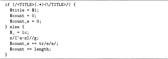
4.6 In section 4.4, the proportions of the letter e in 68 Poe stories are given. Here are some steps to compute these values. First, download the five volumes from the Web, and get rid of the initial and ending text so that just the titles and stories are left. Second, although the titles are easy for a person to read, it helps to make them completely unambiguous. One common way to add information to a text is by XML tags. These work the same way as HTML tags except that they can stand for anything, not just how to display a Web page. Here we put the story titles in between two title tags, for example, <TITLE> The Black Cat</TITLE>. Third, scan these five files line by line using a while loop. Finally, use code sample 4.3 as a start for counting the total number of letters (in $ count) and the number of e’s (in $count_e).
4.7 [Mathematical] For some distributions, the sample data can be summarized by a few sufficient statistics without loss of any information about the population parameters. However, this assumes that the data values are really generated by the assumed population distribution, which is rarely exactly true when working with a real data set. Hence, in practice, reducing the data to sufficient statistics can lose information about how well the population distribution fits the observed data.
Code Sample 4.3 Code sample for problem 4.6.
Here is an example that is discussed in section 9.4.1. Equation 9.1 gives a sequence of 0’s and 1‘s reproduced here as equation 4.12.
(4.12)1111111111110000000011111
Suppose we assume that this sequence is generated by a coin, where 1 stands for heads and 0 for tails. Assume that the probability of heads is p, which we wish to estimate. Assuming that this model is true, then the sufficient statistic for p is estimated by the number of l’s divided by the number of flips, which gives 17/25 = 68%.
However, this data set does not look like it comes from flipping a coin because the 0’s and l’s tend to repeat. For this problem, compute the probability of getting the data in equation 4.12 assuming that a coin with p = 0.68 is, in fact, used.
If this probability is low, then the assumption of a biased coin model is cast into doubt. However, reducing the data set to the sufficient statistic for p makes it impossible to decide on the validity of this coin model; that is, information is lost by ignoring the original data in favor of the estimate p = 0.68.
Hint: see section 9.4.1 for one approach of estimating the probability observing equation 4.12 if seventeen l’s and eight 0’s can appear in any order with equal probability.
For more on sufficient statistics see chapter 10 of Lee Bain and Max Engelhardt’s Introduction to Probability and Mathematical Statistics [7]. In addition, the point that the data set does have more information than the sufficient statistic is made in section 8.7 of John A. Rice’s Mathematical Statistics and Data Analysis [106].
For the normal distribution, the sample mean and sample standard deviation are sufficient for the population mean and population standard deviation. See theorem 7.1.1 of James Press’s Applied Multivariate Analysis [103] for a proof.
4.8 To randomize the words in a story requires two steps. First, they must be identified. Second, they are stored and then permuted. The task of identifying the words is discussed in section 2.4 (and see program 2.6). So here we focus on rearranging them. For each word, store it in a hash using a string generated by the function rand as follows.
$permutation{randO} = $word;
Then print out the hash %permutation by sorting on its keywords (either a numerical or an alphabetical sort works). Since the keywords are randomly generated, the sort randomly permutes the values of this hash.