
Chapter 5: Exponential Smoothing of Nonseasonal Series
5.1 Simple Exponential Smoothing
5.2 Double Exponential Smoothing
5.3 Forecasting Danish Fertility by Exponential Smoothing
5.5 Forecast Errors for the Prediction of Danish Fertility
5.6 Moving Average Representations
5.7 Calculating Confidence Limits for Forecasts
5.8 Applying Confidence Limits for Forecasts
5.9 Confidence Limits for Forecasts of Danish Fertility
5.10 Determining the Smoothing Constant
5.11 Estimating the Smoothing Parameter in PROC ESM
5.12 Holt Exponential Smoothing and the Damped-Trend Method
5.13 Forecasting Fertility by the Damped-Trend Method in PROC ESM
5.14 Concluding Remarks on Exponential Smoothing for Eorecasting
5.1 Simple Exponential Smoothing
When the only purpose of a time series analysis is to produce reliable forecasts based on the history of the series itself, it is often pointless to set up a full statistical model because simple intuitive techniques could often do the job equally well. When applying such methods, no knowledge of statistic or econometric theory is required and the investigator is not forced to make many decisions; only obvious considerations on whether seasonality or trends are present in the series are needed.
In this section, we consider a time series ![]() observed for an equidistant time index t = 1, .., T, and we assume that the only purpose is to construct forecasts
observed for an equidistant time index t = 1, .., T, and we assume that the only purpose is to construct forecasts ![]() of future values of the time series for forecasting horizons i = 1, 2 , 3, . In this and the following section, some theoretical background is presented. See Section 5.3 for the first application using a SAS procedure.
of future values of the time series for forecasting horizons i = 1, 2 , 3, . In this and the following section, some theoretical background is presented. See Section 5.3 for the first application using a SAS procedure.
The technique of exponential smoothing is often applied for forecasting because the idea is simple and very intuitive. Moreover, the technique is easily extended to cover more complicated situations than might be expected at first glance. For this reason, exponential smoothing provides the forecaster with a suitable tool box for most practical forecasting problems. This method has a long history. For an early reference, see Brown (1962).
The idea underlying exponential smoothing is that the series varies around some smooth curve that might be considered as the true, however unobserved, level, which is varying over time. The actual observations apart from this true level consist of irregularities for each particular point in time. When the estimated level is denoted ![]() , the basic formula for updating the level is
, the basic formula for updating the level is
![]()
where α is some smoothing constant 0 < α < 1. In order to start the algorithm, the starting value ![]() is defined as
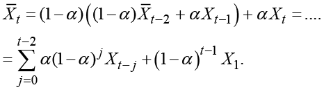
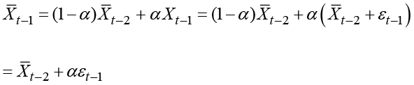
is defined as ![]() .This method is named exponential smoothing because the smoothed series is defined as a weighted average of the observations with exponentially declining weights. The basic formula for this method is easily iterated to
.This method is named exponential smoothing because the smoothed series is defined as a weighted average of the observations with exponentially declining weights. The basic formula for this method is easily iterated to
 .
.
Exponential smoothing defines the estimated true level ![]() at time t as a weighted average of the previous estimated value of the smoothed component
at time t as a weighted average of the previous estimated value of the smoothed component ![]() and the present observed value of the series
and the present observed value of the series ![]() . The smaller the value of α, the smoother the plot of the estimated level
. The smaller the value of α, the smoother the plot of the estimated level ![]() becomes as the present value of the actual observed series is weighted by α. In the extreme situation α = 0, the estimated true value becomes a constant, and for α = 1, no smoothing is performed at all and
becomes as the present value of the actual observed series is weighted by α. In the extreme situation α = 0, the estimated true value becomes a constant, and for α = 1, no smoothing is performed at all and ![]() for all of time t.
for all of time t.
Forecasting past the last observation ![]() is simply performed by defining the prediction as
is simply performed by defining the prediction as
![]()
for all forecasting horizons i. This produces a constant prediction of all future values which, because no external information is included in the forecasting algorithm, could be the best possible forecast.
In many practical situations, forecasting by simple exponential smoothing looks just like forecasting along vertical lines drawn by hand by eyeballing the latest part of the observation period. For this reason, the calculations above seem superfluous and their only justifications are their objectivity and suitability for forecasting. The method requires refinements, as described in the following sections, in situations with trending or seasonal behavior. It turns out that these refinements are easily derived using alternative formulations of the basic formula of exponential smoothing.
5.2 Double Exponential Smoothing
When the series varies along a linear trend, you must modify the procedure. If the basic formula for exponential smoothing is applied to a time series that is an exact linear function, a straight line ![]() , this original linear function is not established. Instead, the smoothing results in data points along a linear function defined by
, this original linear function is not established. Instead, the smoothing results in data points along a linear function defined by
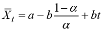
which forms a straight line parallel to the original line.
This is true because the smoothed series ![]() that is defined by this formula meets the difference equation for the smoothed series
that is defined by this formula meets the difference equation for the smoothed series
![]()
Plugging in the original linear function ![]() gives
gives
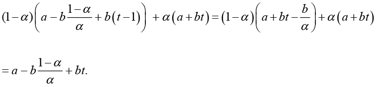
The smoothed series is seen to form a line parallel to the line formed by the observations with a vertical distance given by

which depends only on the slope b and the smoothing constant α. For b > 0, this line is placed below the line formed by the observations with the indicated vertical distance. A correct fit should of course include a shift of this line in order to match the line formed by the observations. This is achieved by iterating the idea of exponential smoothing, introducing the doubled smoothed series ![]() defined by
defined by
![]() .
.
Using the same smoothing constant α. In this way, the smoothed series is smoothed once more, resulting in the double smoothed series ![]() . If the original observations (and thereby also the smoothed values) form straight lines, the double smoothed series
. If the original observations (and thereby also the smoothed values) form straight lines, the double smoothed series ![]() again forms a straight line parallel to and below the two other lines (still for b > 0), with the same vertical distance
again forms a straight line parallel to and below the two other lines (still for b > 0), with the same vertical distance

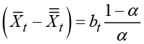
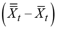
to the line of the single smoothed series ![]() . This means that this vertical distance could be calculated as the difference
. This means that this vertical distance could be calculated as the difference

between the single and the double smoothed series.
In practice, the original observations do not form a strictly linear curve and the calculated vertical distance is time dependent. The slope parameter bt for the linear trend that is calculated at time index t is obtained by solving the equation
 .
.
This formula provides us with the estimate
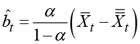
for the slope parameter and the value
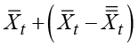
as an estimate for the true level calculated at time t. This estimated level fits the observations in the form of a curve of true levels, which locally forms a linear function of the time index. This idea is appropriate if approximately linear trends, but with varying slopes, are present for longer periods in the time series.
If b < 0, the single smoothed series ![]() forms a parallel line above the line defined by the observations with a vertical distance
forms a parallel line above the line defined by the observations with a vertical distance

while the distance in this situation is estimated by
 .
.
Solving the equation results with the same estimated slope parameter ![]() .
.
These values calculated from the last observed value of the time series form the basis for prediction of future values by
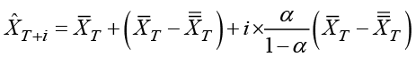 .
.
This idea could be applied once more by defining a triple smoothed process by smoothing the double smoothed series. In this way, an exact quadratic trend could be fitted perfectly. In practice, almost all curved trends could be fitted by triple exponential smoothing because the quadratic curve with parameters fitted for each time index t forms a second-order Taylor approximation to the curve of true levels. However, forecasting by a quadratic curve involves the forecasting horizon i squared, which makes the forecasts tend to explode even for short forecasting horizons. Therefore, in most situations, double exponential smoothing seems more plausible than triple exponential smoothing.
Note that when it comes to practical use of double and triple smoothing, in order to allow for trends in the forecasting procedure, it is in no way necessary to assume that an exact linear trend is present in the data. Only the derived value for the last observation at time index T is used for forecasting. The procedure allows for flexible trends with time-varying slopes. The most recent trend is extrapolated, and the success of the prediction then depends on how long this trend continues in the future.
5.3 Forecasting Danish Fertility by Exponential Smoothing
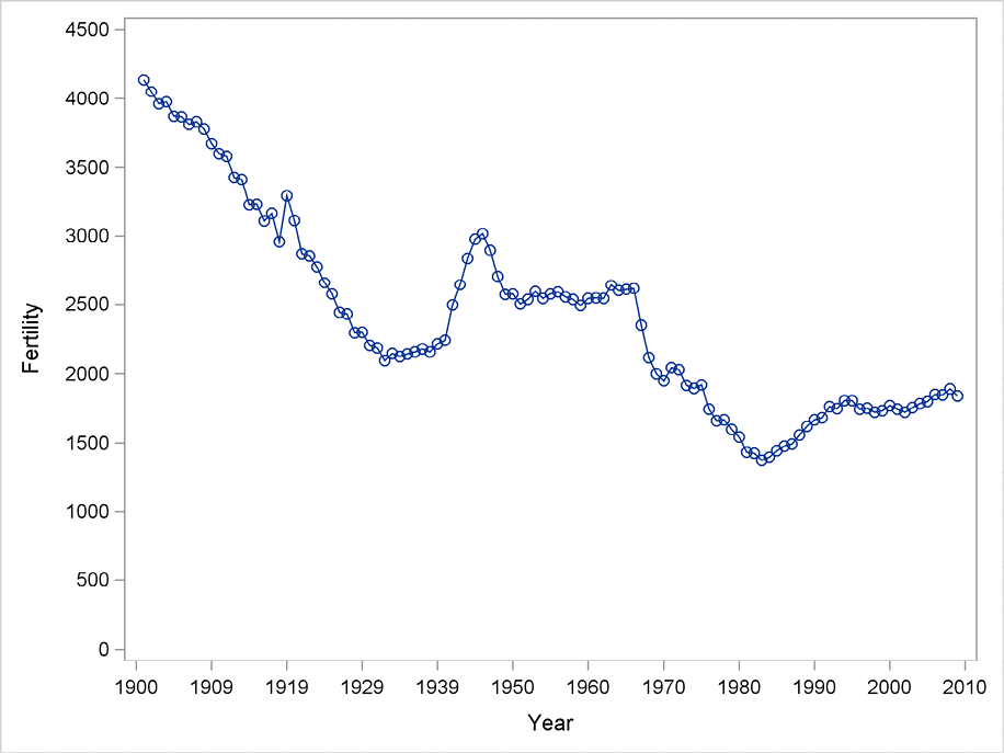
The measure of fertility considered in this example is the expected number of children born of 1000 women in their reproductive years. The series consists of yearly observations for 1901–2009 and is stored in the fertility data set, which contains a variable named fertility. A simple plot of the time series, shown in Figure 5.1, shows that in general, fertility is declining with a perhaps unexpected short peak during the years of World War II. In recent years, however, the level has stabilized, and in fact the trend is recently somewhat slowly upward. The current value of about 1800 states that Danish women on average will have given birth to 1.8 children by the time they reach the age of 50 years. (The economic, social, and demographic explanations for this behavior are outside the scope of this example. You can refer to demographic textbooks for a discussion of such issues.)
Figure 5.1 Number of children borne by 1000 Danish women
A simple application of PROC ESM using exponential forecasting is shown in the following code. The choice of method is simple exponential smoothing, because that is the default. By default, the procedure prints nothing to the output window, but the option print=all requests that all possible output be printed. Usually, this is of minor importance, and for this first example this output is not commented on. The procedure produces lots of graphics using SAS Statistical Graphics, but this example demonstrates how to save these forecasts in a new SAS data set (out) created by the option outfor=out. This data set is saved in the temporary library Work because no library name is specified. The actual observations are stored in this output data set for the whole observation period if they are included in the original data set, but this variable is renamed to actual. The predictions are stored in a variable named predict. For the years up to the starting year of the predictions, the one-step-ahead forecasts are included in the variable predict. These values and the corresponding prediction errors are also included in the output data set. Standard errors and confidence limits for the forecasts are described later in this chapter.
The option back=80 specifies that the model is fitted based only on the first 29 observations up to 1929 because the forecasts period starts 80 years previous to the latest observation, which is 2009. The remaining observations for 1930 and thereafter are kept as a control. For that reason, forecasts for 80 years are calculated by the option lead=80. The time index is stated in the ID statement; in this case the time index is the variable year in the data set Fertility. This variable has to be in a SAS date format as described in Chapter 2, even if the advantages of these formats are unimportant for this yearly series.
Program 5.1 A simple application of PROC ESM
proc esm data=sasts.fertility outfor=out
back=80 lead=80 print=all;
   id year interval=year;
   forecast fertility;
run;
proc sgplot data=out;
series x=year y=actual/ markers;
series x=year y=predict/ markers;
yaxis values=(0 to 4500 by 500);
efline ‘01JUL1929’d / axis=x;
run;
The forecasts in the output data set are then plotted by PROC SGPLOT in Program 5.1. Also, the actual observations are plotted, and the beginning of the forecasting period is marked by a vertical line. Note the variable names actual and predict for the observed values and the predictions in the data set produced by PROC ESM.
For the years 1901–1929, which are applied for fitting the algorithm, the method adapts to a level that is slowly declining. It seems that each forecast almost equals the latest observation. From 1930–2009, the forecasts are based only on the historical values from 1901–1929. The forecasts for the whole period 1930–2009 are constant because no trend is included in this simple exponential smoothing in which forecasts simply form a constant line. By luck, this is a rather successful procedure for most of the forecasting period because the clear downward trend in Danish fertility in fact stopped around 1930.
Figure 5.2 Forecasting the fertility series using simple exponential smoothing
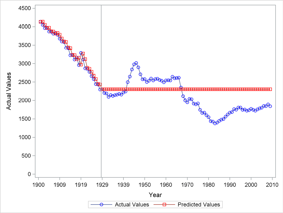
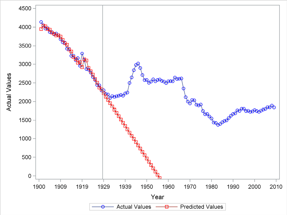
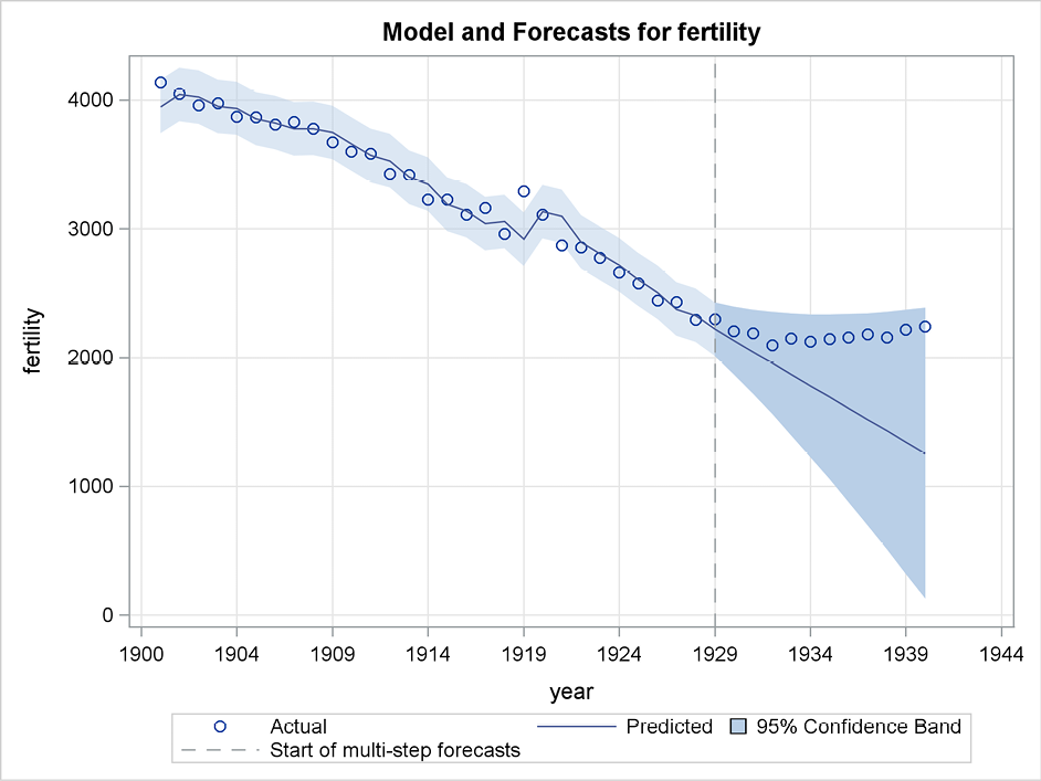
Figure 5.3 gives the same results, but in this case, a linear trend is included by the specification model=double in the FORECAST statement as:
forecast fertility/model=double;
This specifies double exponential smoothing as the forecasting method. The rest of Program 5.1 is unchanged.
In the fitting period, the fit is better than for simple exponential smoothing. The downward trend fits the observed series well in the years 1901 to 1930. This is the case because the one-year-ahead predictions are consistently below the observed value for the previous year and the trend is present, and therefore close to the actual value. But in the forecasting period, the trend for the observed series breaks after a few years, and the forecasts after that break are completely misleading.
Figure 5.3 Forecasting Danish fertility using double exponential smoothing
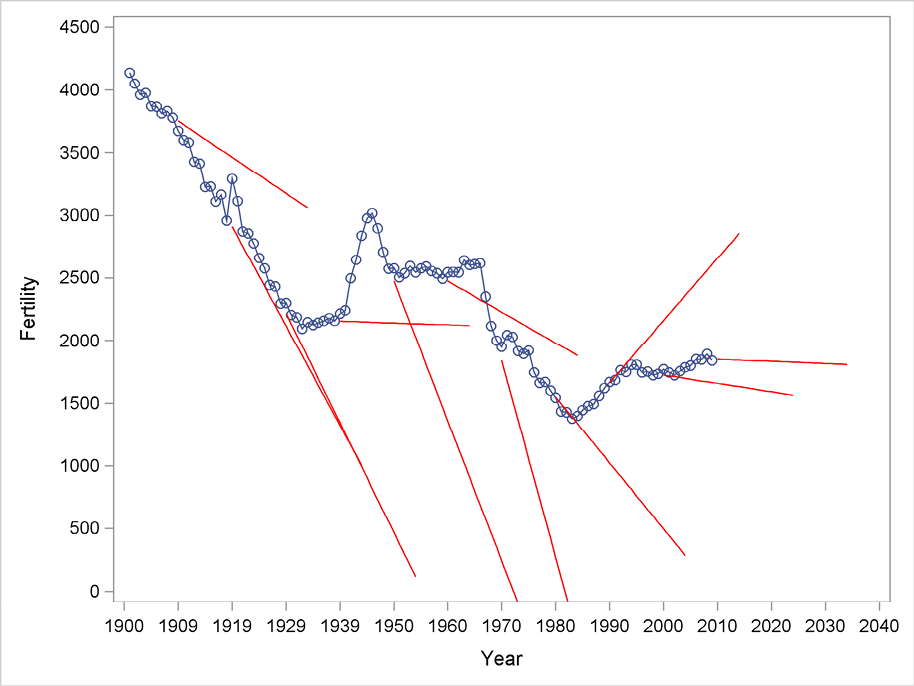
In order to study the forecasting performances of simple and double exponential smoothing methods within periods of different trending behavior, the forecasts are now generated with different starting points. The following plots, using simple exponential smoothing in Figure 5.4 and double exponential smoothing in Figure 5.5, are generated by successive applications of PROC ESM with starting points 1930, 1940, .. , 2010. (This could be done by including in the code a macro with a do-loop, but the details of macro programming are outside the scope of this book. See Burlew [1998] for a discussion of macro programming in SAS.)
Using simple exponential smoothing with no trend, as plotted in Figure 5.4, the forecasting function is constant. This is relevant at starting points where no trend is apparent in the following years, but it is highly misleading at starting points where trends are clearly present. Similarly, the impression from Figure 5.5 when forecasting with double exponential smoothing is that this method is successful for some starting points and highly misleading for others, depending on the future behavior of the trend.
A closer look shows, however, that the predictions using both methods for just one or two years ahead seem appropriate for most of the starting points even if the observations ten years ahead are far from the 10th-horizon forecasts. This means that the forecasting procedure works well for short-term forecasting, but it is hard to tell whether simple or double exponential smoothing performs best.
Figure 5.4 Forecasting using simple exponential smoothing from many starting points
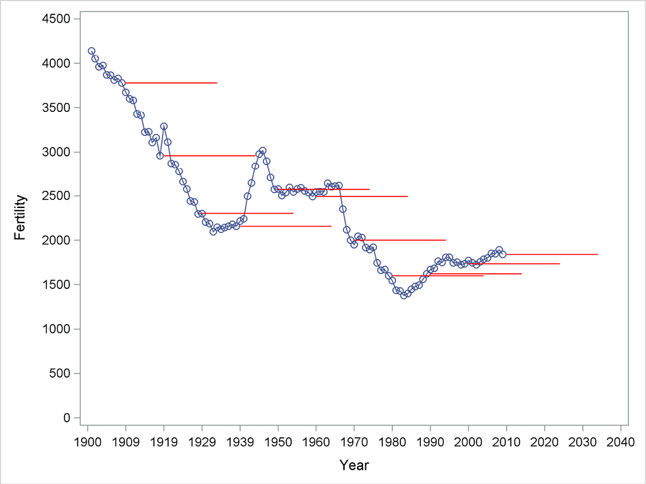
Figure 5.5 Forecasting using double exponential smoothing from many starting points
The main conclusion up to now is that these simple predictions using exponential smoothing are useful as an algorithm for intuitive rule-of-thumb forecasting because they perform well in the short term. But they are valid only when forecasting for longer horizons and the underlying assumptions are valid. Simple exponential smoothing produces good predictions during periods with no systematic trend. Double exponential smoothing is appropriate during periods with a nearly constant trend. But neither method provides you with reliable forecasts as a general method for all starting points.
5.4 Forecast Errors
If observed values are predicted using only past values of the series, actual observations could be compared with the predictions, and the forecast errors could serve as a basis for evaluating the forecasting precision.
For all observations, the actual observation ![]() could be compared with
could be compared with ![]() , which is the prediction of
, which is the prediction of ![]() calculated using only values of the time series up to time index t - 1. The differences between the observed values
calculated using only values of the time series up to time index t - 1. The differences between the observed values ![]() and the predicted values
and the predicted values ![]() form a series of remainder terms, also called residuals, which are considered to be stochastic in statistical modeling of time series. If the forecasting procedure is sufficient, they should vary unsystematically as any systematic behavior indicates further structures in the time series that should be included in order to improve the forecasts.
form a series of remainder terms, also called residuals, which are considered to be stochastic in statistical modeling of time series. If the forecasting procedure is sufficient, they should vary unsystematically as any systematic behavior indicates further structures in the time series that should be included in order to improve the forecasts.
In practice, it is often seen that a plot of the actual observations![]() combined with a plot of the predictions of the time point t based on observations up to time t – 1, here denoted
combined with a plot of the predictions of the time point t based on observations up to time t – 1, here denoted ![]() , looks like two parallel curves for exponential smoothing because the prediction mirrors the previous observation. This is the situation for the years where one-year-ahead predictions are compared with the actual observations shown in Figure 5.2 and to some extent in Figure 5.3 for the Danish fertility series. This is of course a great problem for the prediction, but it is often impossible to prevent, when only information of the observations up to time t - 1 is at hand when predicting
, looks like two parallel curves for exponential smoothing because the prediction mirrors the previous observation. This is the situation for the years where one-year-ahead predictions are compared with the actual observations shown in Figure 5.2 and to some extent in Figure 5.3 for the Danish fertility series. This is of course a great problem for the prediction, but it is often impossible to prevent, when only information of the observations up to time t - 1 is at hand when predicting ![]() .
.
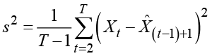
The remainder terms form the basis for the construction of confidence limits for the predictions by considering the remainder terms as Gaussian distributed. The variance of the residuals is usually estimated as the mean square prediction error in the observation period
 .
.
The confidence interval for a prediction that is one time period ahead is then constructed by the usual formula
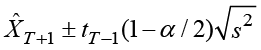
where a Student’s t-distribution quantile is used to correspond to the chosen confidence level α. The degrees of freedom is the length of the time series minus 1, but because the number of observations is usually greater than 30, an approximation by a standard Gaussian distribution could be applied as well. In Section 5.7, confidence limits for predictions with a horizon greater than 1 are constructed.
5.5 Forecast Errors for the Prediction of Danish Fertility
In order to study the validity of the forecasting method, you could plot the remainder terms. The output data set generated by the option also includes the forecast errors for the one-step-ahead predictions for the whole observation period because no back= option is used. This was the case in Program 5.1. In the output data set, the forecast errors are stored in a variable named error. The plot is generated by PROC SGPLOT.
The plot in Figure 5.6 shows all one-period-ahead prediction errors for double exponential smoothing for the whole observation period 1901 to 2009 as the lower curve. The series of actual observations is also displayed as the upper curve on the plot in order to see during which periods the prediction errors are large or small. Prediction errors provide an indication of periods with good forecasting performance and periods for which the method is misleading. It is obvious that this method works well as long as the trend continues, but if the trend changes, it takes a while until the forecasts are back in place again. This is especially obvious in the 1940s.
Program 5.2 Plotting prediction errors
proc esm data=sasts.fertility outfor=out
lead =0 print=all;
   id year interval=year;
   forecast fertility/model=double;
run;
proc sgplot data=out;
series y=actual x=year/ markers;
series y=error x=year/ markers;
yaxis values=(-1000 to 4500 by 500);
refline 0/axis=y;
run;
Figure 5.6 Residuals from double exponential smoothing
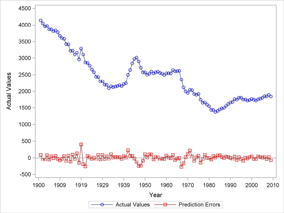
The forecast errors as plotted in Figure 5.6 seem to vary systematically, having the same sign for long periods. This indicates that the predictions are either too high or too small for many successive years. This systematic behavior is called positive autocorrelation by statisticians, and it could be modeled in order to improve the forecasting performance. Chapter 7 will examine this subject in more detail.
5.6 Moving Average Representations
This section provides a first attempt to see exponential smoothing as a specific type of time series model. The conclusion is that more detailed model building is often superfluous if a proper exponential smoothing is applied.
The basic formula for simple exponential smoothing,
![]()
could be considered in the following way. Assume that the forecast error for a prediction that is one time period ahead is considered as a residual ![]() , defined by the difference
, defined by the difference
![]()
or, equivalently,
![]() .
.
Then, it is obtained from the basic formula for exponential smoothing that
and then
![]()
Applying this recursively leads to the expression
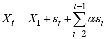 .
.
An obvious application of this formula is the following expression for the forecast error when forecasting for horizon i:
![]()
For double exponential smoothing, similar formulas exist; however, they are more complicated. The result is
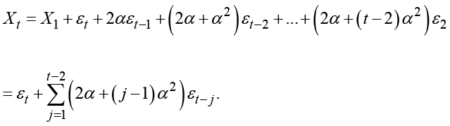
In the theory of time series, the class of moving average models is defined as
![]()
for series of independently identical distributed error terms ![]() , which have mean 0 and variance
, which have mean 0 and variance ![]() . This model is denoted MA(q). Although the representations of the formulas for smoothing the time series do not lead to a finite number of error terms, the application of exponential smoothing forecasting methods can be seen as a kind of fitting a moving average model of high order. This idea is pursued further in Chapter 7, which also includes empirical analyses by special SAS procedures.
. This model is denoted MA(q). Although the representations of the formulas for smoothing the time series do not lead to a finite number of error terms, the application of exponential smoothing forecasting methods can be seen as a kind of fitting a moving average model of high order. This idea is pursued further in Chapter 7, which also includes empirical analyses by special SAS procedures.
5.7 Calculating Confidence Limits for Forecasts
The expression of the forecast error for forecasting with horizon i using simple exponential smoothing in Section 5.4 could be used to derive confidence limits for the forecast function. The variance is:
The confidence limits are then calculated as the square root of this variance times a quantile in the Student’s t-distribution or in the standard normal distribution, that is, 1.96 for the commonly applied 95% confidence level. The confidence limits are seen to grow like the square root function of the forecasting horizon. The underlying assumptions for these results are discussed in Section 5.8.
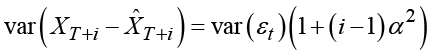
Similarly, it can be seen from the representation for double exponential smoothing in Section 5.2 that the forecast error for forecasting i periods ahead is

meaning that the forecasting variance for double exponential smoothing equals
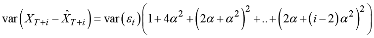 .
.
Considered as a function with the forecasting horizon i, this is, in fact, a polynomial of degree three. The confidence limits that are derived using the square root of this variance are then broadening more than linear. This implies that forecast limits in practice are unrealistically broad even for rather short forecasting horizons.
The main conclusion is that the forecast limits broaden at a fast rate and when methods including a trend are applied, this broadening is at a very fast rate. If forecasting using a method that allows for a trend is applied to series without a significant trend, the forecast limits are especially unrealistic. A forecasting method without a trend might be preferable for such a series. An alternative conclusion could be that the broad confidence limits in the long run indicate that long-term forecasting is not precise even if the short-term forecasts are reliable.
Another way to obtain confidence limits for the forecasting function is to reconsider the setup in a linear regression framework. Simple exponential smoothing corresponds to the estimation of a mean parameter by a weighted average of the observed series. Similarly, double exponential smoothing corresponds to a weighted regression in a regression model with the time index as the independent variable. This is made evident by looking at the autoregressive expansion. (See Section 7.1.) By applying standard regression results, forecast limits could be obtained in this way. This regression approach relies on model assumptions that are different from the model assumptions using the moving average expansion, so the resulting confidence limits are different. It turns out that forecast limits based on the regression approach do not have the tendency of quickly broadening as do confidence limits based on the moving average representation. But even if this is what you want, it might be unrealistic for particular series, and narrow confidence limits could of course be misleading. For a discussion of these considerations, see Brown (1962) and Montgomery and Johnson (1976).
5.8 Applying Confidence Limits for Forecasts
The calculation of confidence limits in Section 5.7 relies upon statistical assumptions that are familiar to everyone with a basic knowledge of, say, regression analysis. In short, the forecast errors should be independent, they should have the same variance, and, in order to specify the confidence level appropriately, they should be normally distributed. In practice, all these assumptions are often doubtful.
The assumption of independence is violated when there is a systematic variation in the signs of the forecast errors. For many time series examples, the series has many level shifts for which the forecast errors tend to have the same sign until the forecast method has adapted to the new situation. Also, a trend break (for example, a break from an upward trend to a constant level) will provide overly high forecasts until the trend component has adapted to the new situation, and forecast errors will be negative for a long sequence of observations. Another phenomenon is outliers caused by changes in the timing in the series, which invalidate the independence assumption. An example of this is a sales series for which low sales one month might be followed with high sales the next month as the consumers merely postpone their buying.
All these examples are indeed series for which the simple forecasting method is inadequate, meaning that the forecasts could be improved. In this section, the lack of independence is mentioned as the only violation of the assumptions behind the construction of confidence limits. A formal testing of the hypothesis is discussed in Chapter 7, which also includes some methods for improving the forecasting of such series with further modeling.
The assumption of equal variances can also be verified by looking at a plot of forecast errors. If the variation tends to decrease or increase in the observation period, the assumption is violated. One remedy is to transform to the series before applying the forecasting method. This is possible using PROC ESM, as described in Section 6.7. It is important to remember that the forecasting performance is not critically relying on the assumption of equal variances, and the forecasts are, in practice, not changing very much if more proper methods are applied. The problem is mainly those forecast limits that systematically become too narrow or too broad due to the unequal variances.
The assumption of normal distributed error terms is seldom met in real-world economic data. Most often, the distribution is more heavy tailed, meaning that the probability of large forecast errors is larger than indicated by the normal distribution, and fewer errors are situated in the middle of the distribution. For this reason, the error variance ![]() becomes large and the confidence limits are broader than expected, indicating pure forecasting performance. When compared with a normal distribution, too many observations are considered to be outliers because the forecast error exceeds twice the standard deviation even if the estimated variance is large due to the many large forecast errors.
becomes large and the confidence limits are broader than expected, indicating pure forecasting performance. When compared with a normal distribution, too many observations are considered to be outliers because the forecast error exceeds twice the standard deviation even if the estimated variance is large due to the many large forecast errors.
The reason is that every observation (apart from a stochastic term, which could be modeled by the normal distribution) includes components that in a formulated statistical model should be considered deterministic. Such deterministic components could be strikes, transport problems, weather conditions, and so on. In proper modeling, these factors are known and as such they should be accounted for by specific outlier modeling. The stochastic error component should include only all truly unknown events, and forecast limits should account for these. Deterministic events are used as explanations (or perhaps excuses) for future forecast errors. The forecast limits calculated by the simple application of the historical forecast error variance are broad. They would include a probability of a future hurricane if the series in the observation period was affected by a hurricane.
When applying such simple forecasting methods, the forecaster could choose not to use more precise statistical time series modeling. This is often a very sensible choice because it seems meaningless to spend lots of effort modeling past values of the time series when the real purpose is to produce forecasts. Of course, all these departures from the forecasting assumptions are opportunities for improving the forecasts, but they could also indicate that the actual series is very hard to forecast properly. The basic assumption in forecasting is that behavior in the past contains information about what will happen in the future. Violation of that assumption is often an indication that proper forecasting is difficult, if not to say impossible, to perform using only past observations of the series itself.
5.9 Confidence Limits for Forecasts of Danish Fertility
Figure 5.7 presents a plot of forecasts for the years 1930 to 2010, generated by Program 5.3. The forecasts in this plot are actually identical to the forecasts in Figure 5.2. The forecasts in Program 5.1 were stored in a new data set and afterward plotted by a plotting procedure. Figure 5.7 is generated by the Statistical Graphics facility in SAS in order to show the plotting possibilities offered by PROC ESM. Statistical Graphics provide an easy way to produce forecast plots with confidence limits. But because the stored data set in Program 5.1 also includes standard deviations and confidence limits for the forecasts, the plot in Figure 5.2 could also be extended by confidence limits.
The option plot=all states that all available plots are generated. The plot in Figure 5.7 is the model and forecast plot, but you can also choose plots for only the forecast period, or select one of many plots on model fit. These plots are discussed later on.
Figure 5.7 shows the forecasts as a simple horizontal line with a confidence band. The confidence band is derived by the moving average representation, which leads to steadily increasing confidence limits. See Section 5.6.
Program 5.3 Plotting forecasts and confidence limits
ods graphics;
proc esm data=sasts.fertility outfor=out
back=80 lead=80 plot=all;
   id year interval=year;
   forecast fertility;
run;
ods graphics off;
Figure 5.7 Confidence limits for forecasting with simple exponential smoothing
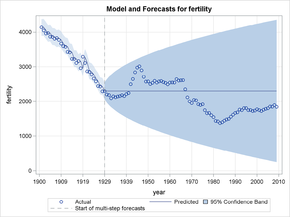
Figure 5.8 similarly shows the forecast of Danish fertility for 1930 and beyond using double exponential smoothing by specifying the following statement:
forecast fertility/model=double;
As the fertility was steadily decreasing in the years up to the latest observation used for this forecasting, the double exponential smoothing algorithm derives only forecasts that continue the trend. Of course, they are misleading in the long run but for about the first four years, they are pretty close to the observed values. The forecast limits are broad, and the lower confidence limit becomes negative after a few years, which stops the produced plot. In fact, the length of the confidence interval is of the order ![]() for the forecast for horizon i (that is, forecasting the fertility i years ahead). These confidence limits could be narrowed to 80% by using the option alpha=0.2 in the procedure statement.
for the forecast for horizon i (that is, forecasting the fertility i years ahead). These confidence limits could be narrowed to 80% by using the option alpha=0.2 in the procedure statement.
Figure 5.8 Confidence limits for forecasts using double exponential smoothing
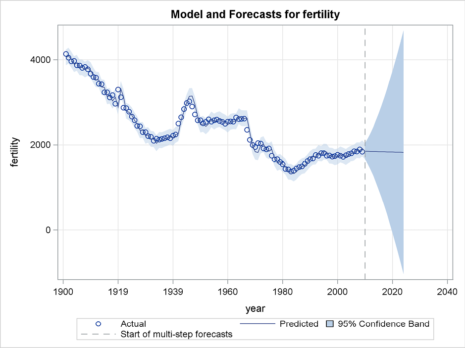
A similar plot of forecasts generated by double exponential smoothing in PROC ESM, using the latest observation for the year 2009 as the starting point, is presented in Figure 5.9. In this situation, the forecasts are calculated after a period with a relatively constant level of Danish fertility. The forecast is rather constant because the trend extracted by the double exponential smoothing is almost zero.
Figure 5.9 Forecast with confidence limits for future observations
5.10 Determining the Smoothing Constant
The success of the various methods of exponential smoothing relies heavily on the choice of the weight α in the smoothing algorithm. A weight parameter α near 0 gives high weight to previous observations and the estimated level. Therefore, the predictions are almost the same for all observations. On the other hand, a value of α near 1 would give heavy weight to the most recent observation, and the predictions would look very volatile.
The weighting parameters can be estimated by minimizing the error sum of squares for the predictions one step ahead
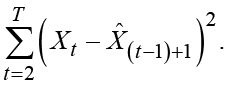
This procedure for estimating the value of the weighting parameter mimics an estimation of a parameter in a Gaussian statistical model. In many ways, it is for that reason a good procedure, and it can be the start of real statistical model building for the time series. But for many practical purposes, it might not be a good idea. The behavior of the time series could vary, and the whole idea behind the application of exponential smoothing for forecasting is to provide forecasts that are robust and that do not rely on rigid assumptions for an underlying statistical model. Practical experience leads to the conclusion that fixed values for the weighting parameters
might do the job just as well as estimated values. This could also reflect the fact that the residual sum of squares is rather flat when considered as a function of the smoothing constants. For that reason, the smoothing constants are not determined very precisely. In statistical terms, this could be seen in the reported standard deviations for the estimated smoothing weights. A consequence is that fixed values for the smoothing constants work just as well as estimated values. The difference is of no practical importance.
5.11 Estimating the Smoothing Parameter in PROC ESM
PROC ESM includes the ability to estimate the weight parameters in applications of exponential smoothing. In Program 5.1, these estimates are printed by adding the additional option print=estimates or print=all, as in Program 5.4 where double exponential smoothing is applied.
Program 5.4 Double exponential smoothing using PROC ESM
ods graphics;
PROC ESM data=sasts.fertility print=estimates plot=all;
id year interval=year;
forecast fertility/method=double alpha=0.2;
run;
ods graphics off;
The weight parameter is estimated to be 0.63, as shown in Output 5.1. This value of the smoothing parameter means that the smoothing gives almost half the weight to the most recent observations and the other half to the past experiences. This parameter value is estimated by using the series for the whole observation period 1901–2009 as the fitting period. The resulting plot is Figure 5.10, which shows 80% confidence limits due to the option alpha=0.2. The forecasts form a straight, almost horizontal, line because the observed values in the latest part of the series are nearly constant.
Output 5.1 Estimates of the smoothing parameter by PROC ESM
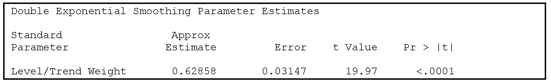
Figure 5.10 Observed values and predictions calculated by PROC ESM
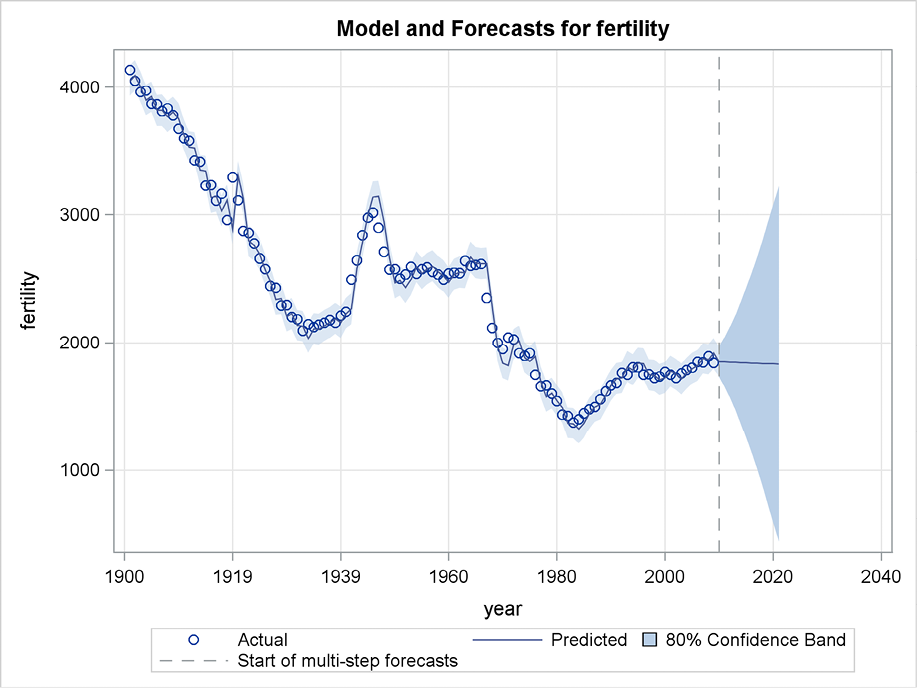
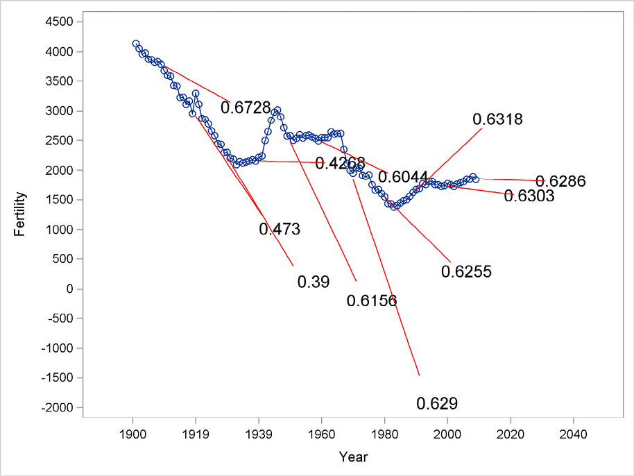
Figure 5.11 presents estimates of this parameter when it is estimated for only a part of the observation period (from the first observation in 1901 up to a varying last observation). The predictions form straight lines with different slopes, and they are the same as the predictions presented in Figure 5.5. The values of the estimated smoothing parameter are around 0.6 for most estimation periods. But for a few periods, the parameter is estimated as 0.4. This happens after periods with a clear linear trend, which corresponds to situations where the past has a larger influence and determines the trend very well.
Figure 5.11 Estimates of the smoothing parameter for various estimation intervals
5.12 Holt Exponential Smoothing and the Damped-Trend Method
An alternative formulation of a trend is to concentrate on the series of increments ![]() , and then estimate the slope parameter of a linear trend by exponential smoothing of these differences. This method was first proposed by Holt (1957). In a series with a linear trend, this should equal the slope of the trend with some added noise specific for the situation at the time index t. The trend slope, which is allowed to be time varying, is denoted
, and then estimate the slope parameter of a linear trend by exponential smoothing of these differences. This method was first proposed by Holt (1957). In a series with a linear trend, this should equal the slope of the trend with some added noise specific for the situation at the time index t. The trend slope, which is allowed to be time varying, is denoted ![]() . The idea is basically to update the true level using the present observation
. The idea is basically to update the true level using the present observation ![]() from the previous level
from the previous level ![]() to
to ![]() by an adjustment to the previous slope element
by an adjustment to the previous slope element ![]() using exponential smoothing. Moreover, the basic formula for exponential smoothing is applied to update from the estimate of
using exponential smoothing. Moreover, the basic formula for exponential smoothing is applied to update from the estimate of ![]() to an estimate of the actual
to an estimate of the actual![]() as an average of the last slope element
as an average of the last slope element ![]() and the present observed increment
and the present observed increment![]() of the estimated true level. Expressed as formulas, these two updating equations then become
of the estimated true level. Expressed as formulas, these two updating equations then become
![]()
and
![]() .
.
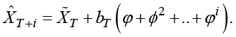
The formula for prediction is
![]()
In this formulation, two weighting parameters (α and γ) are used for the two updating equations. Of course, the same parameter value could also be applied.
This idea of a time-dependent level that includes a time-dependent slope component is developed further in Part 5. The unobserved components models discussed in these chapters form a complete basis for statistical models for the time series, which could be applied to provide more efficient forecasting.
An additional possibility is to develop the idea to the damped-trend methods. As the term “damped-trend” indicates, the trend is reduced when the prediction is for larger horizons i by an exponential declining factor ![]()
Because the prediction for horizon i = 1 is also damped by the factor ![]() (because the trend element is
(because the trend element is ![]() rather than
rather than ![]() ), the updating formulas are adjusted to
), the updating formulas are adjusted to
![]()
and
![]()
The advantage of this method is that when a trend is forecast far into the future, it often takes unnatural values. For instance, a declining linear trend could give an acceptable fit for shorter horizons, but for longer horizons it could take negative values for a series which by definition is supposed to be positive.
If ![]() , the damping effect is none and an ordinary Holt linear exponential smoothing is performed. However,
, the damping effect is none and an ordinary Holt linear exponential smoothing is performed. However, ![]() gives no smoothing at all and the situation
gives no smoothing at all and the situation ![]() is the same as letting both
is the same as letting both ![]() and
and ![]() .
.
5.13 Forecasting Fertility by the Damped-Trend Method in PROC ESM
The observed time series of Danish fertility includes many periods of trends lasting for periods of 5 to 15 years. This fertility series appears to have a local dependence, but information about fertility more than five years back seems to be of little use for forecasting future values. This implies that only short-term prediction is valuable while long-term predictions are pure guesswork and are therefore much better done by common sense ideas about the development of the trend. At the least, forecasts along a linear trend are obviously misleading in the long run even if they could be valuable for short-term forecasting.
By using the damped-trend forecasting method, this behavior could be fitted in order to forecast a few years ahead along the trend without letting the trend continue for the long-run forecasts. The damped-trend method is incorporated in PROC ESM, where the method is simply denoted by method=damptrend,as in Program 5.5. Here the forecasts are calculated at a starting point, 1970, in the middle of a downward-trending period, which makes this forecasting method very successful. See Figure 5.12 for the long-run prediction.
Program 5.5 Damped-trend forecasting using PROC ESM
ods graphics;
PROC ESM data=sasts.fertility print=estimates plot=all back=40 lead=50;
id year interval=year;
forecast fertility/method=damptrend alpha=0.2;
run;
ods graphics off;
Figure 5.12 Forecasting by the damped-trend method using PROC ESM
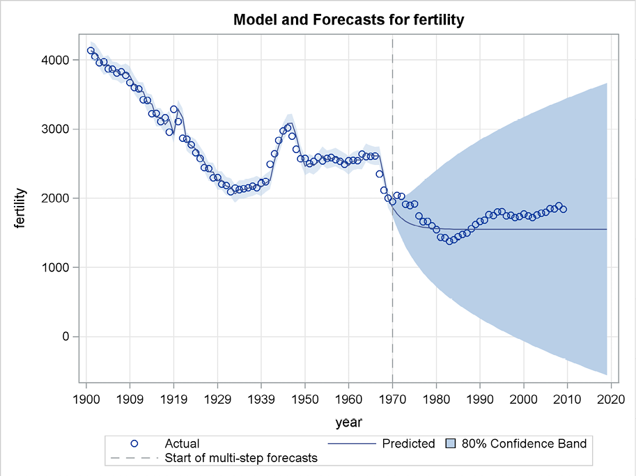
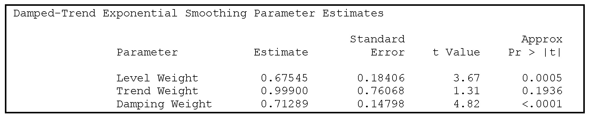
The estimated parameters are written to the output window by the option print=estimates. See Output 5.2. The value 0.71 for the damping coefficient φ is so close to 1 that it allows the trend to dominate the forecasts for many years, but in the long run the forecasting function becomes flat. The smoothing coefficient for the trend equals 1, which means that the trend is determined by the most recently observed one-year increment of the series. The standard deviation for this parameter is large, so values of this smoothing parameter that are less than 1 are also plausible. This is because the local trends are rather constant and the slope coefficient could equally well be estimated by the latest increment or by previously observed increments.
Output 5.2 Smoothing parameters estimated by PROC ESM for the damped-trend method
In Figure 5.13, the forecast errors are plotted for the whole series of observations. The damping coefficient φ is estimated as 0.64 when the complete data series is used. An obvious problem is the outliers around 1920, where fertility suddenly became more volatile, probably due to problems with defining fertility in the years close to the reunion of Southern Jutland after 50 years of German supremacy. This is very apparent in the plot of forecast errors shown in Figure 5.13. Apart from these outliers, the prediction error plot indicates no problems with the model as the errors seem to vary unsystematically. This conclusion is confirmed by the diagnostic plots generated by PROC ESM. Because these plots rely on theory that is covered in later chapters, they will not be discussed here.
Figure 5.13 Residuals for predictions calculated by the damped-trend method
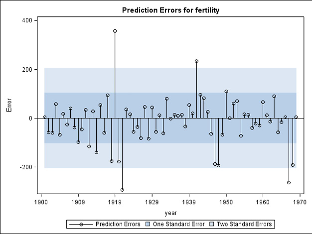
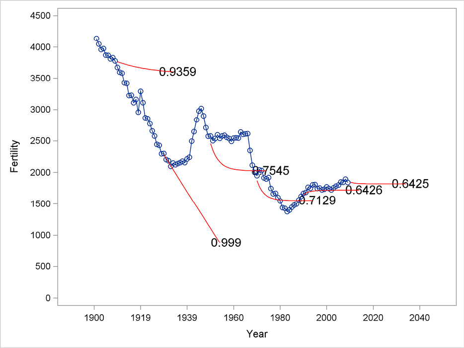
Figure 5.14 presents forecasts by the damped-trend method for many starting points. The plot shows the estimated damping coefficient, φ. For the first starting points and up to 1930, this damping factor is almost 1, meaning that the trend is allowed to continue for many years. The value 0.999 is the largest possible estimated value for the coefficient φ because it is bounded by 1. After 1930, the steady downward trend ends and the damping factors are estimated to values clearly less than 1, with values around φ = 0.7. These values allow a trend for the previous years to continue for some time but the forecasting after a few years becomes flat.
Figure 5.14 Estimated damping coefficients for fitting periods with various ending points
5.14 Concluding Remarks about Exponential Smoothing for Forecasting
This series for Danish fertility is an example of a series that is hard to predict by exponential smoothing methods. The series has a clear downward trend for the first part of the series 1901 to around 1930 for which the level rapidly decreases from approximately 4000 to 2000. This is a difference of close to four down to close to two children born for each Danish woman. For the years after 1930, the level of series varies around 2000. But the level has changed rather rapidly, with a peak of about 3000 in the 1940s to a steady level of about 2500 in the 1950s, and then declining to 1500 in the beginning of the 1980s. For the most recent years, it varies close to 1800.
In the first part of the period, any automatic algorithm for forecasting would assume that the downward trend continues. But knowing the actual definition of the series makes this assumption unrealistic; fertility cannot be negative. For the remaining period, the level is changing and forecasting to some extent has to adjust to the fluctuating level of the series. Adjustment is possible, using the simple exponential smoothing algorithm, but this method cannot incorporate the short trending periods in the observed series. Double exponential smoothing, on the other hand, is very good at catching up trends after a very few years, but it then forecasts along this trend to the infinite future, which of course is unrealistic for this particular time series.
The damped-trend method combines characteristics of both simple exponential smoothing and double exponential smoothing. This algorithm allows a trend observed for a few years to continue, but after a few years the trending behavior in the forecasts diminishes and the forecast becomes constant. Depending on the structure of the series to be forecast, keep these factors in mind when you choose a forecasting method.