
![]()
One of the most difficult transitions to make to become highly proficient at writing SQL well is to shift from thinking procedurally to thinking declaratively (or in sets). It is often hardest to learn to think in sets if you’ve spent time working with virtually any programming language. If this is the case for you, you are likely very comfortable with constructs such as IF-THEN-ELSE, WHILE-DO, LOOP-END LOOP, and BEGIN-END. These constructs support working with logic and data in a very procedural, step-by-step, top-down–type approach. The SQL language is not intended to be implemented from a procedural point of view, but from a set-oriented one. The longer it takes you to shift to a set-oriented point of view, the longer it takes for you to become truly proficient at writing SQL that is functionally correct and also highly optimized to perform well.
In this chapter, we explore common areas where you may need to shift your procedural way of thinking to nonprocedural ways, which allows you to start to understand how to work with sets of data elements vs. sequential steps. We also look at several specific set operations (UNION, INTERSECT, MINUS) and how nulls affect set-thinking.
Using a real-world example as a way to help you start thinking in sets, consider a deck of playing cards. A standard card deck consists of 52 cards, but the deck can be broken into multiple sets as well. How many sets can you make from the main set of standard playing cards? Your answer depends, in part, on any rules that might be applied to how a set is defined. So, for our purposes, let’s say there is only one rule for making a set: All cards in a set must have something in common. With that rule in place, let’s count the sets. There are a total of 22 sets:
- Four sets—one for each suit (diamonds, clubs, spades, hearts)
- Two sets—one for each color (red, black)
- Thirteen sets—one for each individual card (Ace, 2 through 10, Jack, Queen, King)
- One set—face cards only (Jack, Queen, King)
- One set—nonface cards only (Ace, 2 through 10)
You might be able to think up some other sets in addition to the 22 I’ve defined, but you get the idea, right? The idea is that if you think of this example in terms of SQL, there is a table, named DECK, with 52 rows in it. The table could have several indexes on columns by which we intend to filter regularly. For instance, we could create indexes on the suit column (diamonds, clubs, spades, hearts), the color column (red, black), the card_name column (Ace, 2 through 10, Jack, Queen, King), and the card_type column (face card/nonface card). We could write some PL/SQL code to read the table row by row in a looping construct and to ask for different cards (rows) to be returned or we could write a single query that returns the specific rows we want. Which method do you think is more efficient?
Consider the PL/SQL code method. You can open a cursor containing all the rows in the DECK table and then read the rows in a loop. For each row, you check the criteria you want, such as all cards from the suit of hearts. This method requires the execution of 52 fetch calls, one for each row in the table. Then, each row is examined to check the value of the suit column to determine whether it is hearts. If it is hearts, the row is included in the final result; otherwise, it is rejected. This means that out of 52 rows fetched and checked, only 13 are a match. In the end, 75 percent of the rows are rejected. This translates to doing 75 percent more work than absolutely necessary.
However, if you think in sets, you can write a single query, SELECT * FROM DECK WHERE SUIT = 'HEARTS', to solve the problem. Because there is an index on the suit column, the execution of the query uses the index to return only the 13 cards in the suit of hearts. In this case, the query is executed once and there is nothing rejected. Only the rows wanted are accessed and returned.
The point of this example is to help you to think in sets. With something you can actually visualize, like a deck of cards, it seems quite obvious that you should think in sets. It just seems natural. But, if you find it hard to make a set with a deck of cards, I bet you find it harder to think in sets when writing SQL. Writing SQL works under the same premise (set-thinking is a must!); it’s just a different game. Now that you’re warmed up to think in sets, let’s look at several ways to switch procedural thinking to set-thinking.
Moving from Procedural to Set-Based Thinking
The first thing you need to do is to stop thinking about process steps that handle data one row at a time. If you’re thinking one row at a time, your thinking uses phrases such as “for each row, do x” or “while value is y, do x.” Try to shift this thinking to use phrases such as “for all.” A simple example of this is adding numbers. When you think procedurally, you think of adding the number value from one row to the number value from another row until you’ve added all the rows together. Thinking of summing all rows is different. This is a very simple example, but the same shift in thinking applies to situations that aren’t as obvious.
For example, if I asked you to produce a list of all employees who spent the same number of years in each job they held within the company during their employment, how would you do it? If you think procedurally, you look at each job position, compute the number of years that position was held, and compare it with the number of years any other positions were held. If the number of years don’t match, you reject the employee from the list. This approach might lead to a query that uses a self-join, such as the following:
select distinct employee_id
  from job_history j1
 where not exists
       (select null
          from job_history j2
         where j2.employee_id = j1.employee_id
           and round(months_between(j2.start_date,j2.end_date)/12,0) <>
                round(months_between(j1.start_date,j1.end_date)/12,0) )
On the other hand, if you look at the problem from a set-based point of view, you might write the query by accessing the table only once, grouping rows by employee, and filtering the result to retain only those employees whose minimum years in a single position match their maximum years in a single position, like this:
select employee_id
  from job_history
 group by employee_id
having min(round(months_between(start_date,end_date)/12,0)) =
max(round(months_between(start_date,end_date)/12,0))
Listing 4-1 shows the execution of each of these alternatives. You can see that the set-based approach uses fewer logical reads and has a more concise plan that accesses the job_history table only once instead of twice.
Listing 4-1. Procedural vs. Set-Based Approach
SQL> select distinct employee_id
  2    from job_history j1
  3   where not exists
  4         (select null
  5            from job_history j2
  6           where j2.employee_id = j1.employee_id
  7             and round(months_between(j2.start_date,j2.end_date)/12,0) <>
  8                 round(months_between(j1.start_date,j1.end_date)/12,0) );

    EMPLOYEE_ID
---------------
            102
            201
            114
            176
            122

--------------------------------------------------------------
| Id  | Operation           | Name        | A-Rows | Buffers |
--------------------------------------------------------------
|   0 | SELECT STATEMENT    |             |      5 |      14 |
|   1 |  HASH UNIQUE        |             |      5 |      14 |
|*  2 |   HASH JOIN ANTI    |             |      6 |      14 |
|   3 |    TABLE ACCESS FULL| JOB_HISTORY |     10 |       7 |
|   4 |    TABLE ACCESS FULL| JOB_HISTORY |     10 |       7 |
--------------------------------------------------------------

Predicate Information (identified by operation id):
---------------------------------------------------

   2 - access("J2"."EMPLOYEE_ID"="J1"."EMPLOYEE_ID")
       filter(ROUND(MONTHS_BETWEEN(INTERNAL_FUNCTION("J2"."START_DATE"),
       INTERNAL_FUNCTION("J2"."END_DATE"))/12,0)<>
       ROUND(MONTHS_BETWEEN(INTERNAL_FUNCTION("J1"."START_DATE"),
       INTERNAL_FUNCTION("J1"."END_DATE"))/12,0))

SQL> select employee_id
  2    from job_history
  3   group by employee_id
  4  having min(round(months_between(start_date,end_date)/12,0)) =
  5        max(round(months_between(start_date,end_date)/12,0));

    EMPLOYEE_ID
---------------
            102
            114
            122
            176
            201

------------------------------------------------------------------------
| Id  | Operation                     | Name        | A-Rows | Buffers |
------------------------------------------------------------------------
|   0 | SELECT STATEMENT              |             |      5 |       4 |
|*  1 |  FILTER                       |             |      5 |       4 |
|   2 |   SORT GROUP BY NOSORT        |             |      7 |       4 |
|   3 |    TABLE ACCESS BY INDEX ROWID| JOB_HISTORY |     10 |       4 |
|   4 |     INDEX FULL SCAN           | JHIST_PK    |     10 |       2 |
------------------------------------------------------------------------

Predicate Information (identified by operation id):
---------------------------------------------------

   1 - filter(MIN(ROUND(MONTHS_BETWEEN(INTERNAL_FUNCTION("START_DATE"),
          INTERNAL_FUNCTION("END_DATE"))/12,0))=MAX(ROUND(MONTHS_BETWEEN(
          INTERNAL_FUNCTION("START_DATE"),INTERNAL_FUNCTION("END_DATE"))
          /12,0)))
The key is to start thinking in terms of completed results, not process steps. Look for group characteristics and not individual steps or actions. In set-based thinking, everything exists in a state defined by the filters or constraints applied to the set. You don’t think in terms of process flow but in terms of the state of the set. Figure 4-1 shows a comparison between a process flow diagram and a nested sets diagram to illustrate my point.
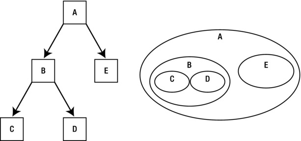
Figure 4-1. A process flow diagram vs. a nested set diagram
The process flow diagram implies the result set (A) is achieved through a series of steps that build on one another to produce the final answer. B is built by traversing C and D, and then A is built by traversing B and E. However, the nested sets diagram views A as a result of a combination of sets.
Another common but erroneous way of thinking is to consider tables to be ordered sets of rows. Just think of how you typically see table contents listed. They’re shown in a grid or spreadsheet-type view. However, a table represents a set, and a set has no order. Showing tables in a way that implies a certain order can be confusing. Remember from Chapter 2 that the ORDER BY clause is applied last when a SQL statement is executed. SQL is based on set theory, and because sets have no predetermined order to their rows, order has to be applied separately after the rows that satisfy the query result have been extracted from the set. Figure 4-2 shows a more correct way to depict the content of tables that doesn’t imply order.
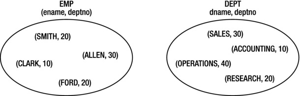
Figure 4-2. The EMP and DEPT sets
It may not seem important to make these seemingly small distinctions in how you think, but these small shifts are fundamental to understanding SQL correctly. Let’s look at an example of writing a SQL statement taking both a procedural thinking approach and a set-based approach to help clarify the distinctions between the two.
Procedural vs. Set-Based Thinking: An Example
In this example, the task is to compute an average number of days between orders for a customer. Listing 4-2 shows one way to do this from a procedural thinking approach. To keep the example output shorter, I work with one customer only, but I could convert this easily to handle all customers.
Listing 4-2. Procedural Thinking Approach
SQL> -- Show the list of order dates for customer 102
SQL> select customer_id, order_date
  2  from orders
  3  where customer_id = 102 ;

    CUSTOMER_ID ORDER_DATE
--------------- -------------------------------
            102 19-NOV-99 06.41.54.696211 PM
            102 14-SEP-99 11.53.40.223345 AM
            102 29-MAR-99 04.22.40.536996 PM
            102 14-SEP-98 09.03.04.763452 AM
SQL>
SQL> -- Determine the order_date prior to the current row’s order_date
SQL> select customer_id, order_date,
  2             lag(order_date,1,order_date)
  3             over (partition by customer_id order by order_date)
  4             as prev_order_date
  5  from orders
  6  where customer_id = 102;

    CUSTOMER_ID ORDER_DATE                       PREV_ORDER_DATE
--------------- -------------------------------- ----------------------------
            102 14-SEP-98 09.03.04.763452 AM     14-SEP-98 09.03.04.763452 AM
            102 29-MAR-99 04.22.40.536996 PM     14-SEP-98 09.03.04.763452 AM
            102 14-SEP-99 11.53.40.223345 AM     29-MAR-99 04.22.40.536996 PM
            102 19-NOV-99 06.41.54.696211 PM     14-SEP-99 11.53.40.223345 AM
SQL>
SQL> -- Determine the days between each order
SQL> select trunc(order_date) - trunc(prev_order_date)  days_between
  2  from
  3  (
  4  select customer_id, order_date,
  5             lag(order_date,1,order_date)
  6             over (partition by customer_id order by order_date)
  7             as prev_order_date
  8  from orders
  9  where customer_id = 102
 10  );

   DAYS_BETWEEN
---------------
              0
            196
            169
             66
SQL>
SQL> -- Put it together with an AVG function to get the final answer
SQL> select avg(trunc(order_date) - trunc(prev_order_date))  avg_days_between
  2  from
  3  (
  4  select customer_id, order_date,
  5             lag(order_date,1,order_date)
  6             over (partition by customer_id order by order_date)
  7             as prev_order_date
  8  from orders
  9  where customer_id = 102
 10  );

AVG_DAYS_BETWEEN
----------------
          107.75
This looks pretty elegant, doesn’t it? In this example, I executed several queries one by one to show you how my thinking follows a step-by-step procedural approach to writing the query. Don’t worry if you’re unfamiliar with the use of the analytic function LAG; analytic functions are covered in Chapter 8. Briefly, what I’ve done is to read each order row for customer 102 in order by order_date and, using the LAG function, look back at the prior order row to get its order_date. When I have both dates—the date for the current row’s order and the date for the previous row’s order—it’s a simple matter to subtract the two to get the days in between. Last, I use the average aggregate function to get my final answer.
You can tell that this query is built following a very procedural approach. The best giveaway to knowing the approach is the way I can walk through several different queries to show how the final result set is built. I can see the detail as I go along. When you’re thinking in sets, you find that you don’t really care about each individual element. Listing 4-3 shows the query written using a set-based thinking approach.
Listing 4-3. Set-Based Thinking Approach
SQL> select (max(trunc(order_date)) - min(trunc(order_date))) / count(*) as avg_days_between
  2  from orders
  3  where customer_id = 102 ;

AVG_DAYS_BETWEEN
----------------
          107.75
How about that? I really didn’t need anything fancy to solve the problem. All I needed to compute the average days between orders was the total duration of time between the first and last order, and the number of orders placed. I didn’t need to go through all that step-by-step thinking as if I was writing a program that would read the data row by row and compute the answer. I just needed to shift my thinking to consider the problem in terms of the set of data as a whole.
I do not discount the procedural approach completely. There may be times when you have to take that approach to get the job done. However, I encourage you to shift your thinking. Start by searching for a set-based approach and move toward a more procedural approach only when and to the degree needed. By doing this, you likely find that you can come up with simpler, more direct, and often better performing solutions.
Set Operations
Oracle supports four set operators: UNION, UNION ALL, MINUS, and INTERSECT. Set operators combine the results from two or more SELECT statements to form a single result set. This differs from joins in that joins are used to combine columns from each joined table into one row. The set operators compare completed rows between the input queries and return a distinct set of rows. The exception to this is the use of UNION ALL, which returns all rows from both sets, including duplicates. UNION returns a result set from all input queries with no duplicates. MINUS returns distinct rows that appear in the first input query result but not in the subsequent ones. INTERSECT returns the distinct rows that appear in all input queries.
All queries that are used with set operators must conform to the following conditions:
- All input queries must retrieve the same number of columns.
- The data types of each column must match the corresponding column (by order in the column list) for each of the other input queries. It is possible for data types not to match directly, but only if the data types of all input queries can be converted implicitly to the data types of the first input query.
- The ORDER BY clause may not be used in the individual queries and may only be used at the end of the query, where it applies to the entire result of the set operation.
- Column names are derived from the first input query.
Each input query is processed separately and then the set operator is applied. Last, the ORDER BY is applied to the total result set if one is specified. When using UNION and INTERSECT, the operators are commutative (in other words, the order of the queries doesn’t matter). However, when using MINUS, the order is important because this set operation uses the first input query result as the base for comparison with other results. All set operations except for UNION ALL require that the result set go through a sort/distinct process that means additional overhead to process the query. If you know that no duplicates ever exist, or you don’t care whether duplicates are present, make sure to use UNION ALL.
UNION and UNION ALL are used when the results of two or more separate queries need to be combined to provide a single, final result set. Figure 4-3 uses Venn diagrams to show how the result set for each type can be visualized.
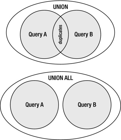
Figure 4-3. Venn diagram for UNION and UNION ALL result sets
The UNION set operation returns the results of both queries but removes duplicates whereas the UNION ALL returns all rows including duplicates. As mentioned previously, in cases when you need to eliminate duplicates, use UNION. But, when either you don’t care if duplicates exist or you don’t expect duplicates to occur, choose UNION ALL. Using UNION ALL has a less resource-intensive footprint than using UNION because UNION ALL does not have to do any processing to remove duplicates. This processing can be quite expensive in terms of both resources and response time to complete. Prior to Oracle version 10, a sort operation was used to remove duplicates. Beginning with version 10, an option to use a HASH UNIQUE operation to remove duplicates is available. The HASH UNIQUE doesn’t sort, but uses hash value comparisons instead. I mention this to make sure you realize that even if the result set appears to be in sorted order, the result set is not guaranteed to be sorted unless you explicitly include an ORDER BY clause. UNION ALL avoids this “distincting” operation entirely, so it is best to use it whenever possible. Listing 4-4 shows examples of using UNION and UNION ALL.
Listing 4-4. UNION and UNION ALL Examples
SQL> CREATE TABLE table1 (
  2    id_pk INTEGER NOT NULL PRIMARY KEY,
  3    color VARCHAR(10) NOT NULL);
SQL> CREATE TABLE table2 (
  2    id_pk INTEGER NOT NULL PRIMARY KEY,
  3    color VARCHAR(10) NOT NULL);
SQL> CREATE TABLE table3 (
  2    color VARCHAR(10) NOT NULL);
SQL> INSERT INTO table1 VALUES (1, 'RED'),
SQL> INSERT INTO table1 VALUES (2, 'RED'),
SQL> INSERT INTO table1 VALUES (3, 'ORANGE'),
SQL> INSERT INTO table1 VALUES (4, 'ORANGE'),
SQL> INSERT INTO table1 VALUES (5, 'ORANGE'),
SQL> INSERT INTO table1 VALUES (6, 'YELLOW'),
SQL> INSERT INTO table1 VALUES (7, 'GREEN'),
SQL> INSERT INTO table1 VALUES (8, 'BLUE'),
SQL> INSERT INTO table1 VALUES (9, 'BLUE'),
SQL> INSERT INTO table1 VALUES (10, 'VIOLET'),
SQL> INSERT INTO table2 VALUES (1, 'RED'),
SQL> INSERT INTO table2 VALUES (2, 'RED'),
SQL> INSERT INTO table2 VALUES (3, 'BLUE'),
SQL> INSERT INTO table2 VALUES (4, 'BLUE'),
SQL> INSERT INTO table2 VALUES (5, 'BLUE'),
SQL> INSERT INTO table2 VALUES (6, 'GREEN'),
SQL> COMMIT;
SQL>
SQL> select color from table1
  2  union
  3  select color from table2;

COLOR
----------
BLUE
GREEN
ORANGE
RED
VIOLET
YELLOW

6 rows selected.

SQL> select color from table1
  2  union all
  3  select color from table2;

COLOR
----------
RED
RED
ORANGE
ORANGE
ORANGE
YELLOW
GREEN
BLUE
BLUE
VIOLET
RED
RED
BLUE
BLUE
BLUE
GREEN

16 rows selected.

SQL> select color from table1;

COLOR
----------
RED
RED
ORANGE
ORANGE
ORANGE
YELLOW
GREEN
BLUE
BLUE
VIOLET

10 rows selected.

SQL> select color from table3;

no rows selected

SQL> select color from table1
  2  union
  3  select color from table3;

COLOR
----------
BLUE
GREEN
ORANGE
RED
VIOLET
YELLOW

6 rows selected.

SQL> -- The first query will return a differen number of columns than the second
SQL> select * from table1
  2  union
  3  select color from table2;
select * from table1
*
ERROR at line 1:
ORA-01789: query block has incorrect number of result columns
These examples demonstrate the UNION of two queries. Keep in mind that you can have multiple queries that are “unioned” together.
MINUS
MINUS is used when the results of the first input query are used as the base set from which the other input query result sets are subtracted to end up with the final result set. The use of MINUS has often been used instead of using NOT EXISTS (antijoin) queries. The problem being solved is something like, “I need to return the set of rows that exists in row source A but not in row source B.” Figure 4-4 uses a Venn diagram to show how the result set for this operation can be visualized.
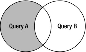
Figure 4-4. Venn diagram for MINUS result sets
Listing 4-5 shows examples of using MINUS.
Listing 4-5. MINUS Examples
SQL> select color from table1
  2  minus
  3  select color from table2;

COLOR
----------
ORANGE
VIOLET
YELLOW

3 rows selected.

SQL> -- MINUS queries are equivalent to NOT EXISTS queries
SQL> select distinct color from table1
  2  where not exists (select null from table2 where table2.color = table1.color) ;

COLOR
----------
ORANGE
VIOLET
YELLOW

3 rows selected.

SQL>
SQL> select color from table2
  2  minus
  3  select color from table1;

no rows selected

SQL> -- MINUS using an empty table
SQL> select color from table1
  2  minus
  3  select color from table3;

COLOR
----------
BLUE
GREEN
ORANGE
RED
VIOLET
YELLOW

6 rows selected.
INTERSECT
INTERSECT is used to return a distinct set of rows that appear in all input queries. The use of INTERSECT has often been used instead of using EXISTS (semijoin) queries. The problem being solved is something like, “I need to return the set of rows from row source A only if a match exists in row source B.” Figure 4-5 uses a Venn diagram to show how the result set for this operation can be visualized.
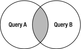
Figure 4-5. Venn diagram for INTERSECT result sets
Listing 4-6 shows examples of using INTERSECT.
Listing 4-6. INTERSECT Examples
SQL> select color from table1
  2  intersect
  3  select color from table2;

COLOR
----------
BLUE
GREEN
RED

3 rows selected.

SQL> select color from table1
  2  intersect
  3  select color from table3;

no rows selected
You often hear the term null value, but in truth, a null isn’t a value at all. A null is, at best, a marker. I always think of null as meaning “I don’t know.” The SQL language handles nulls in unintuitive ways—at least from my point of view; results from their use are often not what I expect in terms of real-world functionality.
IS THE TERM NULL VALUE WRONG?
Strictly speaking, a null is not a value, but rather is the absence of a value. However, the term null value is in wide use. Work in SQL long enough and you surely encounter someone who pontificates on how wrong it is to use the term null value.
But is it really wrong to use the term null value?
If you find yourself on the receiving end of such a lecture, feel free to argue right back. The term null value is widely used in both the ANSI and ISO editions of the SQL standard. Null value is an official part of the description of the SQL language and thus is fair game for use when discussing the language.
Keep in mind, though, that there is a distinction to be drawn between the SQL language and relational theory. A really picky person can argue for the use of “null value” when speaking of SQL, and yet argue against that very same term when speaking of relational theory, on which SQL is loosely based.
Listing 4-7 shows a simple query for which I expect a certain result set but end up with something different than my expectations. I expect that if I query for the absence of a specific value and no matches are found, including when the column contains a null, Oracle should return that row in the result set.
Listing 4-7. Examples Using NULL
SQL> -- select all rows from emp table
SQL> select * from scott.emp ;

  EMPNO ENAME      JOB           MGR HIREDATE     SAL   COMM  DEPTNO
------- ---------- --------- ------- --------- ------ ------ -------
   7369 SMITH      CLERK        7902 17-DEC-80    800             20
   7499 ALLEN      SALESMAN     7698 20-FEB-81   1600    300      30
   7521 WARD       SALESMAN     7698 22-FEB-81   1250    500      30
   7566 JONES      MANAGER      7839 02-APR-81   2975             20
   7654 MARTIN     SALESMAN     7698 28-SEP-81   1250   1400      30
   7698 BLAKE      MANAGER      7839 01-MAY-81   2850             30
   7782 CLARK      MANAGER      7839 09-JUN-81   2450             10
   7788 SCOTT      ANALYST      7566 19-APR-87   3000             20
   7839 KING       PRESIDENT         17-NOV-81   5000
   7844 TURNER     SALESMAN     7698 08-SEP-81   1500      0      30
   7876 ADAMS      CLERK        7788 23-MAY-87   1100             20
   7900 JAMES      CLERK        7698 03-DEC-81    950             30
   7902 FORD       ANALYST      7566 03-DEC-81   3000             20
   7934 MILLER     CLERK        7782 23-JAN-82   1300             10

14 rows selected.

SQL> -- select only rows with deptno of 10, 20, 30
SQL> select * from scott.emp where deptno in (10, 20, 30) ;

  EMPNO ENAME      JOB           MGR HIREDATE     SAL   COMM  DEPTNO
------- ---------- --------- ------- --------- ------ ------ -------
   7369 SMITH      CLERK        7902 17-DEC-80    800             20
   7499 ALLEN      SALESMAN     7698 20-FEB-81   1600    300      30
   7521 WARD       SALESMAN     7698 22-FEB-81   1250    500      30
   7566 JONES      MANAGER      7839 02-APR-81   2975             20
   7654 MARTIN     SALESMAN     7698 28-SEP-81   1250   1400      30
   7698 BLAKE      MANAGER      7839 01-MAY-81   2850             30
   7782 CLARK      MANAGER      7839 09-JUN-81   2450             10
   7788 SCOTT      ANALYST      7566 19-APR-87   3000             20
   7844 TURNER     SALESMAN     7698 08-SEP-81   1500      0      30
   7876 ADAMS      CLERK        7788 23-MAY-87   1100             20
   7900 JAMES      CLERK        7698 03-DEC-81    950             30
   7902 FORD       ANALYST      7566 03-DEC-81   3000             20
   7934 MILLER     CLERK        7782 23-JAN-82   1300             10

13 rows selected.

SQL> -- select only rows with deptno not 10, 20, 30
SQL> select * from scott.emp where deptno not in (10, 20, 30) ;

no rows selected

SQL> -- select only rows with deptno not 10, 20, 30 or null
SQL> select * from scott.emp where deptno not in (10, 20, 30)
  2       or deptno is null;

  EMPNO ENAME      JOB           MGR HIREDATE     SAL   COMM  DEPTNO
------- ---------- --------- ------- --------- ------ ------ -------
   7839 KING       PRESIDENT         17-NOV-81   5000

1 row selected.
This listing demonstrates what is frustrating to me about nulls: They don’t get included unless specified explicitly. In my example, 13 of the 14 rows in the table have deptno 10, 20, or 30. Because there are 14 total rows in the table, I expect a query that asks for rows that do not have a deptno of 10, 20, or 30 to then show the remaining one row. But, I’m wrong in expecting this, as you can see from the results of the query. If I include explicitly the condition also to include where deptno is null, I get the full list of employees that I expect.
I realize what I’m doing when I think this way is considering nulls to be “low values.” I suppose it’s the old COBOL programmer in me that remembers the days when LOW-VALUES and HIGH-VALUES were used. I also suppose that my brain wants to make nulls equate with an empty string. But, no matter what my brain wants to make of them, nulls are nulls. Nulls do not participate in comparisons. Nulls can’t be added, subtracted, multiplied, or divided by anything. If they are, the return value is null. Listing 4-8 demonstrates this fact about nulls and how they participate in comparisons and expressions.
Listing 4-8. NULLs in Comparisons and Expressions
SQL> select * from scott.emp where deptno is null ;

  EMPNO ENAME      JOB           MGR HIREDATE     SAL   COMM  DEPTNO
------- ---------- --------- ------- --------- ------ ------ -------
   7839 KING       PRESIDENT         17-NOV-81   5000

1 row selected.

SQL>
SQL> select * from scott.emp where deptno = null ;

no rows selected

SQL> select sal, comm, sal + comm as tot_comp
  2  from scott.emp where deptno = 30;

   SAL   COMM        TOT_COMP
------ ------ ---------------
  1600    300            1900
  1250    500            1750
  1250   1400            2650
  2850
  1500      0            1500
   950

6 rows selected.
So, when my brain wants rows with a null deptno to be returned in the query from Listing 4-7, I have to remind myself that when a comparison is made with a null, the answer is always “I don’t know.” It’s the same as you asking me if there is orange juice in your refrigerator and me answering, “I don’t know.” You might have orange juice there or you might not, but I don’t know. So, I can’t answer in any different way and be truthful.
The relational model is based on two-value logic (TRUE, FALSE), but the SQL language allows three-value logic (TRUE, FALSE, UNKNOWN)—and this is where the problem comes in. With that third value in the mix, your SQL returns the “correct” answer as far as how three-value logic considers the comparison, but the answers may not be correct in terms of what you expect in the real world. In the example in Listing 4-8, the answer of “no rows selected” is correct in that, because one deptno column contains a null, you can’t know one way or the other if the column might possibly be something other than 10, 20, or 30. To answer truthfully, the answer has to be UNKNOWN. It’s just like me knowing whether you have orange juice in your refrigerator!
So, you have to make sure you keep the special nature of nulls in mind when you write SQL. If you’re not vigilant in watching out for nulls, you’ll very likely have SQL that returns the wrong answer. At least it is wrong as far as the answer you expect.
NULL Behavior in Set Operations
Set operations treat nulls as if they are able to be compared using equality checks. This is an interesting, and perhaps unexpected, behavior given the previous discussion. Listing 4-9 shows how nulls are treated when used in set operations.
Listing 4-9. NULLs and Set Operations
SQL> select null from dual
  2  union
  3  select null from dual
  4  ;

N
-

1 row selected.

SQL> select null from dual
  2  union all
  3  select null from dual
  4  ;

N
-

2 rows selected.

SQL> select null from dual
  2  intersect
  3  select null from dual;

N
-

1 row selected.

SQL> select null from dual
  2  minus
  3  select null from dual;

no rows selected

SQL> select 1 from dual
  2  union
  3  select null from dual;

              1
---------------
              1
2 rows selected.

SQL> select 1 from dual
  2  union all
  3  select null from dual;

              1
---------------
              1
2 rows selected.

SQL> select 1 from dual
  2  intersect
  3  select null from dual ;

no rows selected

SQL> select 1 from dual
  2  minus
  3  select null from dual ;

              1
---------------
              1

1 row selected.
In the first example, when you have two rows with nulls that are “unioned,” you end up with only one row, which implies that the two rows are equal to one another and, therefore, when the union is processed, the duplicate row is excluded. As you can see, the same is true for how the other set operations behave, so keep in mind that set operations treat nulls as equals.
NULLs and GROUP BY and ORDER BY
Just as in set operations, the GROUP BY and ORDER BY clauses process nulls as if they are able to be compared using equality checks. Notice that with both grouping and ordering, nulls are always placed together, just like known values. Listing 4-10 shows an example of how nulls are handled in the GROUP BY and ORDER BY clauses.
Listing 4-10. NULLs and GROUP BY and ORDER BY
SQL> select comm, count(*) ctr
  2  from scott.emp
  3  group by comm ;

  COMM             CTR
------ ---------------
                    10
  1400               1
   500               1
   300               1
     0               1
5 rows selected.
SQL> select comm, count(*) ctr
  2  from scott.emp
  3  group by comm
  4  order by comm ;

  COMM             CTR
------ ---------------
     0               1
   300               1
   500               1
  1400               1
                    10
5 rows selected.
SQL> select comm, count(*) ctr
  2  from scott.emp
  3  group by comm
  4  order by comm
  5  nulls first ;

  COMM             CTR
------ ---------------
                    10
     0               1
   300               1
   500               1
  1400               1
5 rows selected.

SQL> select ename, sal, comm
  2  from scott.emp
  3  order by comm, ename ;

ENAME         SAL   COMM
---------- ------ ------
TURNER       1500      0
ALLEN        1600    300
WARD         1250    500
MARTIN       1250   1400
ADAMS        1100
BLAKE        2850
CLARK        2450
FORD         3000
JAMES         950
JONES        2975
KING         5000
MILLER       1300
SCOTT        3000
SMITH         800

14 rows selected.
The first two examples show the behavior of nulls within a GROUP BY clause. Because the first query returns the result in what appears to be descending sorted order by the comm column, I want to issue the second query to make a point that I made earlier in the book: The only way to ensure order is to use an ORDER BY clause. Just because the first query result appears to be in a sorted order doesn’t mean it is. When I add the ORDER BY clause in the second query, the null group moves to the bottom. In the last ORDER BY example, note that the nulls are displayed last. This is not because nulls are considered to be “high values”; it is because the default for ordered sorting is to place nulls last. If you want to display nulls first, you simply add the clause NULLS FIRST after your ORDER BY clause, as shown in the third example.
This same difference in the treatment of nulls with some operations such as set operations, grouping, and ordering also applies to aggregate functions. When nulls are present in columns that have aggregate functions such as SUM, COUNT, AVG, MIN, or MAX applied to them, they are removed from the set being aggregated. If the set that results is empty, then the aggregate returns a null.
An exception to this rule involves the use of the COUNT aggregate function. The handling of nulls depends on whether the COUNT function is formulated using a column name or a literal (such as * or 1). Listing 4-11 demonstrates how aggregate functions handle nulls.
Listing 4-11. NULLs and Aggregate Functions
SQL> select count(*) row_ct, count(comm) comm_ct,
  2         avg(comm) avg_comm, min(comm) min_comm,
  3         max(comm) max_comm, sum(comm) sum_comm
  4  from scott.emp ;

  ROW_CT  COMM_CT AVG_COMM MIN_COMM MAX_COMM SUM_COMM
-------- -------- -------- -------- -------- --------
      14        4      550        0     1400     2200

1 row selected.
Notice the difference in the value for COUNT(*) and COUNT(comm). Using * produces the answer of 14, which is the total of all rows, whereas using comm produces the answer of 4, which is only the number of nonnull comm values. You can also verify easily that nulls are removed prior to the computation of AVG, MIN, MAX, and SUM because all the functions produce an answer. If nulls aren’t removed, the answers are all null.
Summary
Thinking in sets is a key skill to master to write SQL that is easier to understand and that typically performs better than SQL written from a procedural approach. When you think procedurally, you attempt to force the SQL language, which is nonprocedural, to function in ways it shouldn’t need to function. In this chapter, we examined these two approaches and discussed how to begin to shift your thinking from procedural to set based. As you proceed through the rest of the book, work to keep a set-based approach in mind. If you find yourself thinking row by row in a procedural fashion, stop and check yourself. The more you practice, the easier it becomes.