
![]()
The MODEL clause introduced in Oracle Database version 10g provides an elegant method to replace the spreadsheet. With the MODEL clause, it is possible to use powerful features such as aggregation, parallelism, and multidimensional, multivariate analysis in SQL statements. If you enjoy working with Excel spreadsheets to calculate formulas, you will enjoy working with the MODEL clause, too.
With the MODEL clause, you build matrixes (or a model) of data with a variable number of dimensions. The model uses a subset of the available columns from the tables in your FROM clause and has to contain at least one dimension, at least one measure, and, optionally, one or more partitions. You can think of a model as a spreadsheet file containing separate worksheets for each calculated value (measures). A worksheet has an x- and a y-axis (two dimensions), and you can imagine having your worksheets split up in several identical areas, each for a different attribute (partition).
When your model is defined, you create rules that modify your measure values. These rules are the keys of the MODEL clause. With just a few rules, you can perform complex calculations on your data and even create new rows as well. The measure columns are now arrays that are indexed by the dimension columns, in which the rules are applied to all partitions of this array. After all rules are applied, the model is converted back to traditional rows.
In situations when the amount of data to be processed is small, the interrow referencing and calculating power of the spreadsheet is sufficient to accomplish the task at hand. However, scalability of such a spreadsheet as a data warehouse application is limited and cumbersome. For example, spreadsheets are generally limited to two or three dimensions, and creating spreadsheets with more dimensions is a manually intensive task. Also, as the amount of data increases, the execution of formulas slows down in a spreadsheet. Furthermore, there is an upper limit on the number of rows in a spreadsheet workbook.
Because the MODEL clause is an extension to the SQL language application, it is highly scalable, akin to Oracle Database’s scalability. Multidimensional, multivariate calculations over millions of rows, if not billions of rows, can be implemented easily with the Model clause, unlike with spreadsheets. Also, many database features such as object partitioning and parallel execution can be used effectively with the MODEL clause, thereby improving scalability even further.
Aggregation of the data is performed inside the RDBMS engine, avoiding costly round-trip calls, as in the case of the third-party data warehouse tools. Scalability is enhanced further by out-of-the-box parallel processing capabilities and query rewrite facilities.
The key difference between a conventional SQL statement and the MODEL clause is that the MODEL clause supports interrow references, multicell references, and cell aggregation. It is easier to understand the MODEL clause with examples, so I introduce the MODEL clause with examples, then conclude my discussion by reviewing some of the advanced features in the MODEL clause.
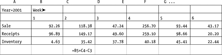
Let’s consider the spreadsheet in Listing 9-1. In this spreadsheet, the inventory for a region and week is calculated using a formula: Current inventory is the sum of last week’s inventory and the quantity received in this week less the quantity sold in this week. This formula is shown in the example using Excel spreadsheet notation. For example, the formula for week 2’s inventory is =B5+C4-C3, where B5 is the prior week’s inventory, C4 is the current week’s receipt_qty, and C3 is the current week’s sales_qty. Essentially, this formula uses an interrow reference to calculate the inventory.
Listing 9-1. Spreadsheet Formula to Calculate Inventory
Product = Xtend Memory, Country ='Australia'
Although it’s easy to calculate this formula for a few dimensions using a spreadsheet, it’s much more difficult to perform these calculations with more dimensions. Performance suffers as the amount of data increases in the spreadsheet. These issues can be remedied by using the Model clause that Oracle Database provides. Not only does the MODEL clause provide for efficient formula calculations, but the writing of multidimensional, multivariate analysis also becomes much more practical.
Interrow Referencing Via the MODEL Clause
In a conventional SQL statement, emulating the spreadsheet described in Listing 9-1 is achieved by a multitude of self-joins. With the advent of the MODEL clause, you can implement the spreadsheet without self-joins because the MODEL clause provides interrow referencing ability.
Example Data
To begin our investigation of the MODEL clause, let’s create a denormalized fact table using the script in Listing 9-2. All the tables referred to in this chapter refer to the objects in SH schema supplied by the Oracle Corporation example scripts.
Listing 9-2. Denormalized sales_fact Table
drop table sales_fact;
CREATE table sales_fact AS
SELECT country_name country,country_subRegion region, prod_name product,
calendar_year year, calendar_week_number week,
SUM(amount_sold) sale,
sum(amount_sold*
  ( case
         when mod(rownum, 10)=0 then 1.4
         when mod(rownum, 5)=0 then 0.6
         when mod(rownum, 2)=0 then 0.9
         when mod(rownum,2)=1 then 1.2
         else 1
    end )) receipts
FROM sales, times, customers, countries, products
WHERE sales.time_id = times.time_id AND
sales.prod_id = products.prod_id AND
sales.cust_id = customers.cust_id AND
customers.country_id = countries.country_id
GROUP BY
country_name,country_subRegion, prod_name, calendar_year, calendar_week_number;
Anatomy of a MODEL Clause
To understand how the MODEL clause works, let’s review a SQL statement intended to produce a spreadsheetlike listing that computes an inventory value for each week of each year in our sales_fact table. Listing 9-3 shows a SQL statement using the MODEL clause to emulate the functionality of the spreadsheet discussed earlier. Let’s explore this SQL statement in detail. We’ll look at the columns declared in the MODEL clause and then we examine rules.
Listing 9-3. Inventory Formula Calculation Using the MODEL Clause
  col product format A30
  col country format A10
  col region format A10
  col year format 9999
  col week format 99
  col sale format 999999
  set lines 120 pages 100

  1    select product, country, year, week, inventory, sale, receipts
  2    from sales_fact
  3    where country in ('Australia') and product ='Xtend Memory'
  4    model return updated rows
  5    partition by (product, country)
  6    dimension by (year, week)
  7    measures ( 0 inventory , sale, receipts)
  8    rules automatic order(
  9         inventory [year, week ] =
 10             nvl(inventory [cv(year), cv(week)-1 ] ,0)
 11           - sale[cv(year), cv(week) ] +
 12           + receipts [cv(year), cv(week) ]
 13     )
 14*   order by product, country,year, week

PRODUCT      COUNTRY     YEAR WEEK  INVENTORY       SALE   RECEIPTS
------------ ---------- ----- ---- ---------- ---------- ----------
..
Xtend Memory Australia   2001    1      4.634      92.26      96.89
Xtend Memory Australia   2001    2     35.424     118.38     149.17
Xtend Memory Australia   2001    3     37.786      47.24      49.60
...
Xtend Memory Australia   2001    9     77.372      92.67     108.64
Xtend Memory Australia   2001   10     56.895      69.05      48.57
..
In Listing 9-3, line 3 declares that this statement is using the MODEL clause with the keywords MODEL RETURN UPDATED ROWS . In a SQL statement using the MODEL clause, there are three groups of columns: partitioning columns, dimension columns, and measures columns. Partitioning columns are analogous to a sheet in the spreadsheet. Dimension columns are analogous to row tags (A, B, C, . . . ) and column tags (1, 2, 3, . . . ). The measures columns are analogous to cells with formulas.
Line 5 identifies the columns product and country as partitioning columns with the clause partition by (product, country). Line 6 identifies columns year and week as dimension columns with the clause dimension by (year, week). Line 7 identifies columns inventory, sales, and receipts as measures columns with the clause measures (0 inventory, sale, receipts). A rule is similar to a formula, and one such rule is defined in lines 8 through 13.
In a mathematical sense, the MODEL clause is implementing partitioned arrays. Dimension columns are indexes into array elements. Each array element, also called a cell, is a measures column.
All rows with the same value for the partitioning column or columns are considered to be in a partition. In this example, all rows with the same value for product and country are in a partition. Within a partition, the dimension columns identify a row uniquely. Rules implement formulas to derive the measures columns and they operate within a partition boundary, so partitions are not mentioned explicitly in a rule.
![]() Note It is important to differentiate between partitioning columns in the MODEL clause and the object partitioning feature. Although you can use the keyword partition in the MODEL clause as well, it’s different from the object partitioning scheme used to partition large tables.
Note It is important to differentiate between partitioning columns in the MODEL clause and the object partitioning feature. Although you can use the keyword partition in the MODEL clause as well, it’s different from the object partitioning scheme used to partition large tables.
Rules
Let’s revisit the rules section from Listing 9-3. You can see both the rule and the corresponding formula together in Listing 9-4. The formula accesses the prior week’s inventory to calculate the current week’s inventory, so it requires an interrow reference. Note that there is a great similarity between the formula and the rule.
Listing 9-4. Rule and Formula
Formula for inventory:

Inventory for (year, week)  = Inventory (year, prior week)
                            - Quantity sold in this week
                            + Quantity received in this week

Rule from the SQL:

  8         inventory [year, week ] =
  9                         nvl(inventory [cv(year), cv(week)-1 ] ,0)
 10                       - sale[cv(year), cv(week) ] +
 11                       + receipts [cv(year), cv(week) ]
The SQL statement in Listing 9-4 introduces a useful function named CV. CV stands for current value and it can be used to refer to a column value in the right-hand side of the rule from the left-hand side of the rule. For example, cv(year) refers to the value of the year column from the left-hand side of the rule. If you think of a formula when it is being applied to a specific cell in a spreadsheet, the CV function allows you to reference the index values for that cell.
Let’s discuss rules with substituted values, as in Listing 9-5. Let’s say that a row with (year, week) column values of (2001, 3) is being processed. The left-hand side of the rule has the values of (2001, 3) for the year and column. The cv(year) clause in the right-hand side of the rule refers to the value of the year column from the left-hand side of the rule—that is, 2001. Similarly, the clause cv(week) refers to the value of the week column from the left-hand side of the rule—that is, 3. So, the clause inventory [cv(year), cv(week)-1] returns the value of the inventory measures for the year equal to 2001 and the prior week (in other words, week 2).
Listing 9-5. Rule Example
Rule example:
 1  rules (
 2      inventory [2001 , 3] = nvl(inventory [cv(year), cv(week)-1 ] ,0)
 3                                 - sale [cv(year), cv(week) ] +
 4                                 + receipts [cv(year), cv(week) ]
 5   )

  rules (
       inventory [2001 , 3] = nvl(inventory [2001, 3-1 ] ,0)
                                  - sale [2001, 3 ] +
                                  + receipts [2001, 3 ]
                            = 35.42  – 47.24 + 49.60
                            = 37.78
  )
Similarly, clauses sale[cv(year), cv(week) ] and receipts[cv(year), cv(week)] are referring to the sale and receipts column values for the year equal to 2001 and the week equal to 3 using the cv function.
Notice that the partitioning columns product and country are not specified in these rules. Rules refer implicitly to the column values for the product and country columns in the current partition.
Positional and Symbolic References
As discussed previously, the cv function provides the ability to refer to a single cell. It is also possible to refer to an individual cell or group of cells using positional or symbolic notations. In addition, you can write FOR loops as a way to create or modify many cells in an arraylike fashion.
Positional notation provides the ability to insert a new cell or update an existing cell in the result set. If the referenced cell exists in the result set, then the cell value is updated; if the cell doesn’t exist, then a new cell is added. This concept of “update if exists, insert if not” is called the UPSERT feature, a fused version of the update and insert facilities. Positional notation provides UPSERT capability.
Suppose that you need to add new cells to initialize the column values for the year equal to 2002 and the week equal to 1. You could achieve this with a rule defined using positional notation. In Listing 9-6, lines 13 and 14 add new cells for the year equal to 2002 and the week equal to 1 using the positional notation with the clause sale[2002,1]=0. Within the square brackets, the position of the value refers to the column order declared in the dimension clause. In this case, column order is (year, week), hence the clause sale[2002,1] refers to the sale column value for the row satisfying the predicates year=2002 and week=1. There are no rows with a column value of year equal to 2002 and week equal to 1, and a new row was inserted with a 0 value for the sale column for the year equal to 2002 and the week equal to 1. The last row in the output was inserted by this rule.
Listing 9-6. Positional Reference to Initialize for Year 2002: UPSERT
  1    select product, country, year, week, inventory, sale, receipts
  2    from sales_fact
  3    where country in ('Australia') and product ='Xtend Memory'
  4    model return updated rows
  5    partition by (product, country)
  6    dimension by (year, week)
  7    measures ( 0 inventory , sale, receipts)
  8    rules automatic order(
  9         inventory [year, week ] =
 10                   nvl(inventory [cv(year), cv(week)-1 ] ,0)
 11                 - sale[cv(year), cv(week) ] +
 12                 + receipts [cv(year), cv(week) ],
 13         sale [2002, 1] = 0,
 14         receipts [2002,1] =0
 15     )
 16*   order by product, country,year, week
...

PRODUCT      COUNTRY     YEAR WEEK  INVENTORY       SALE   RECEIPTS
------------ ---------- ----- ---- ---------- ---------- ----------
...
Xtend Memory Australia   2001   49      2.519      45.26      47.33
Xtend Memory Australia   2001   50     11.775      23.14      32.40
Xtend Memory Australia   2001   51    -20.617     114.82      82.43
Xtend Memory Australia   2001   52    -22.931      23.14      20.83
Xtend Memory Australia   2002    1          0        .00        .00
...
Symbolic notation provides the ability to specify a range of values in the left-hand side of a rule. Let’s say you want to update the sale column values to 110 percent of their actual value for the weeks 1, 52, and 53 for the years 2000 and 2001. The SQL in Listing 9-7 does this. The clause year in (2000,2001) in line 9 uses an IN operator to specify a list of values for the year column. Similarly, the clause week in (1,52,53) specifies a list of values for the week column.
Listing 9-7. Symbolic Reference: UPDATE
  1    select product, country, year, week, sale
  2    from sales_fact
  3    where country in ('Australia') and product ='Xtend Memory'
  4    model return updated rows
  5    partition by (product, country)
  6    dimension by (year, week)
  7    measures ( sale)
  8    rules(
  9      sale [ year in (2000,2001), week in (1,52,53) ] order by year, week
 10           = sale [cv(year), cv(week)] * 1.10
 11    )
 12*   order by product, country,year, week

PRODUCT      COUNTRY     YEAR WEEK       SALE
------------ ---------- ----- ---- ----------
Xtend Memory Australia   2000    1      51.37
Xtend Memory Australia   2000   52      74.20
Xtend Memory Australia   2001    1     101.49
Xtend Memory Australia   2001   52      25.45
Note that the output in Listing 9-7 is not a partial output and that there are no rows for the week equal to 53. Even though you specified 53 in the list of values for the week column in line 9, there are no rows returned for that week. The reason is that symbolic notation can only update the existing cells; it does not allow new cells to be added.
![]() Note I discuss a method to insert an array of cells in the upcoming section “FOR Loops.”
Note I discuss a method to insert an array of cells in the upcoming section “FOR Loops.”
There are no data with a week column value equal to 53 and no new row was added or updated in the result set for the week equal to 53. The ability to generate rows is a key difference between symbolic notation and positional notation. Symbolic notation provides an UPDATE-only facility and positional notation provides an UPSERT facility.
There are a few subtle differences between the SQL statement in Listing 9-7 and prior SQL statements. For example, the statement in Listing 9-7 is missing automatic order in line 8. I discuss the implication of this in the “Rule Evaluation Order” section later in this chapter.
FOR Loops
FOR loops allow you to specify a list of values in the left-hand side of a rule. FOR loops can be defined in the left-hand side of the rule only to add new cells to the output; they can’t be used in the right-hand side of the rule. Syntax for the FOR loop is as follows:
FOR dimension FROM <value1> TO <value2>
[INCREMENT | DECREMENT] <value3>
For example, let’s say you want to add cells for the weeks ranging from 1 to 53 for the year 2002, and initialize those cells with a value of 0. Line 13 in Listing 9-8 inserts new rows for the year 2002 and weeks ranging from 1 to 53 using a FOR loop. Clause Increment 1 increments the week column values to generate weeks from 1 to 53. Similarly, the receipts column is initialized using the clause receipts [2002, for week from 1 to 53 increment 1] =0.
Listing 9-8. Positional Reference, Model, and FOR Loops
  1    select product, country, year, week, inventory, sale, receipts
  2    from sales_fact
  3    where country in ('Australia') and product ='Xtend Memory'
  4    model return updated rows
  5    partition by (product, country)
  6    dimension by (year, week)
  7    measures ( 0 inventory , sale, receipts)
  8    rules automatic order(
  9         inventory [year, week ] =
 10                                   nvl(inventory [cv(year), cv(week)-1 ] ,0)
 11                                    - sale[cv(year), cv(week) ] +
 12                                    + receipts [cv(year), cv(week) ],
 13         sale [ 2002, for week from 1 to 53 increment 1] = 0,
 14         receipts [ 2002,for week from 1 to 53 increment 1] =0
 15     )
 16*   order by product, country,year, week

PRODUCT      COUNTRY     YEAR WEEK  INVENTORY       SALE   RECEIPTS
------------ ---------- ----- ---- ---------- ---------- ----------
...
Xtend Memory Australia   2001   52    -22.931      23.14      20.83
Xtend Memory Australia   2002    1          0        .00        .00
...
Xtend Memory Australia   2002   52          0        .00        .00
Xtend Memory Australia   2002   53          0        .00        .00
...
Returning Updated Rows
In Listing 9-7, just four rows were returned even though there are rows for other weeks. The clause RETURN UPDATED ROWS controls this behavior and provides the ability to limit the cells returned by the SQL statement. Without this clause, all rows are returned regardless of whether the rules update the cells. The rule in Listing 9-7 updates only four cells and other cells are untouched, and so just four rows are returned.
What happens if you don’t specify the clause return updated rows? Listing 9-9 shows the output without the RETURN UPDATED ROWS clause. The output in this listing shows that both updated and nonupdated rows are returned from the SQL statement. The rule updates cells for weeks 1, 52, and 53 only, but the output rows in Listing 9-9 show rows with other column values such as 2, 3, and 4, too.
Listing 9-9. SQL without RETURN UPDATED ROWS
  1    select product, country, year, week, sale
  2    from sales_fact
  3    where country in ('Australia') and product ='Xtend Memory'
  4    model
  5    partition by (product, country)
  6    dimension by (year, week)
  7    measures ( sale)
  8    rules(
  9      sale [ year in (2000,2001), week in (1,52,53) ] order by year, week
 10           = sale [cv(year), cv(week)] * 1.10
 11    )
 12*   order by product, country,year, week

PRODUCT      COUNTRY     YEAR WEEK       SALE
------------ ---------- ----- ---- ----------
...
Xtend Memory Australia   2000   50      21.19
Xtend Memory Australia   2000   52      74.20
Xtend Memory Australia   2001    1     101.49
Xtend Memory Australia   2001    2     118.38
Xtend Memory Australia   2001    3      47.24
Xtend Memory Australia   2001    4     256.70
...
The clause RETURN UPDATED ROWS is applicable to statements using positional notation as well. In Listing 9-10, a rule using a positional notation is shown, inserting a row. Note there are more rows in the table matching with the predicate country in ('Australia') and product ='Xtend Memory'. But, just one row is returned because only one cell is inserted by the rule in line 9. Essentially, the RETURN UPDATED ROWS clause is a limiting clause; it only fetches the rows modified by the rule.
Listing 9-10. RETURN UPDATED ROWS and UPSERT
  1    select product, country, year, week, sale
  2    from sales_fact
  3    where country in ('Australia') and product ='Xtend Memory'
  4    model return updated rows
  5    partition by (product, country)
  6    dimension by (year, week)
  7    measures ( sale)
  8    rules(
  9                 sale [2002, 1] = 0
 10    )
 11*   order by product, country,year, week

PRODUCT      COUNTRY     YEAR WEEK       SALE
------------ ---------- ----- ---- ----------
Xtend Memory Australia   2002    1        .00
Evaluation Order
Multiple rules can be specified in the rules section, and the rules can be specified with dependencies among them. The rule evaluation sequence can affect the functional behavior of the SQL statement, as you will see in this section. Furthermore, even within a single rule, the evaluation of the rule must adhere to a logical sequence. I discuss intrarule valuation order first, then interrule evaluation.
Let’s look at row evaluation order within a rule. Listing 9-11 is copied from Listing 9-3. However, this time, I’ve commented out the keywords AUTOMATIC ORDER in line 8. By commenting these keywords, I force the default behavior of SEQUENTIAL ORDER.
Listing 9-11. Sequential order with Error ORA-32637
 1    select product, country, year, week, inventory, sale, receipts
 2    from sales_fact
 3    where country in ('Australia')
 4    model return updated rows
 5    partition by (product, country)
 6    dimension by (year, week)
 7    measures ( 0 inventory , sale, receipts)
 8    rules  -- Commented: automatic order
 9     (
10         inventory [year, week ] =
11                    nvl(inventory [cv(year), cv(week)-1 ] ,0)
12                  - sale[cv(year), cv(week) ] +
13                  + receipts [cv(year), cv(week) ]
14     )
15*   order by product, country,year, week
       *
ERROR at line 2:
ORA-32637: Self cyclic rule in sequential order MODEL
The rule has an interrow reference with the clause inventory [cv(year), cv(week)-1 ]. Inventory column values must be calculated in ascending order of the week. For example, the inventory rule for week 40 must be evaluated before evaluating the inventory rule for week 41. With AUTOMATIC ORDER, the database engine identifies the row dependencies and evaluates the rows in strict dependency order. Without the AUTOMATIC ORDER clause, row evaluation order is undetermined, which leads to ORA-32637 errors, as shown in Listing 9-11.
It is a better practice to specify the row evaluation order explicitly to avoid this error. Listing 9-12 provides an example. In the rule section, we can specify the order of row evaluation using an ORDER BY year, week clause. This clause specifies that rules must be evaluated in the ascending order of year, week column values. That is, the inventory rule for the year equal to 2000 and the week equal to 40 must be evaluated before evaluating the inventory rule for the year equal to 2000 and the week equal to 41.
Listing 9-12. Evaluation Order at the Cell Level
  1    select product, country, year, week, inventory, sale, receipts
  2    from sales_fact
  3    where country in ('Australia')
  4    model return updated rows
  5    partition by (product, country)
  6    dimension by (year, week)
  7    measures ( 0 inventory , sale, receipts)
  8    rules (
  9         inventory [year, week ] order by year, week =
 10                                   nvl(inventory [cv(year), cv(week)-1 ] ,0)
 11                                    - sale[cv(year), cv(week) ] +
 12                                    + receipts [cv(year), cv(week) ]
 13     )
 14*   order by product, country,year, week

PRODUCT      COUNTRY     YEAR WEEK  INVENTORY       SALE   RECEIPTS
------------ ---------- ----- ---- ---------- ---------- ----------
...
Xtend Memory Australia   2001   49      2.519      45.26      47.33
Xtend Memory Australia   2001   50     11.775      23.14      32.40
...
Note there is no consistency check performed to determine whether this specification of row evaluation order is consistent logically. It is up to the coder—you!—to understand the implications of evaluation order. For example, the row evaluation order in Listing 9-13 is specified with the DESC keyword. Although the rule is syntactically correct, semantic correctness is only known to the coder. Semantic correctness might well require the specification of ASC for an ascending sort. Only the person writing the SQL statement can know which order meets the business problem being addressed.
Listing 9-13. Evaluation Order using the DESC Keyword
 1    select product, country, year, week, inventory, sale, receipts
 2    from sales_fact
 3    where country in ('Australia') and product in ('Xtend Memory')
 4    model return updated rows
 5    partition by (product, country)
 6    dimension by (year, week)
 7    measures ( 0 inventory , sale, receipts)
 8    rules (
 9         inventory [year, week ] order by year, week desc  =
10                     nvl(inventory [cv(year), cv(week)-1 ] ,0)
11                   - sale[cv(year), cv(week) ] +
12                   + receipts [cv(year), cv(week) ]
13     )
14*   order by product, country,year, week

PRODUCT      COUNTRY     YEAR WEEK  INVENTORY       SALE   RECEIPTS
------------ ---------- ----- ---- ---------- ---------- ----------
...
Xtend Memory Australia   2001   49      2.068      45.26      47.33
Xtend Memory Australia   2001   50      9.256      23.14      32.40
...
Notice that inventory column values are different between the Listings 9-12 and 9-13. You need to ensure that the order of row evaluation is consistent with the requirements.
In addition to the order in which rows are evaluated, you also have the issue of the order in which the rules are applied. In Listing 9-14, there are two rules with an interdependency between them. The first rule is evaluating the rule, and it refers to the receipts column, which is calculated by the second rule. These two rules can be evaluated in any order, and the results depend on the order of rule evaluation. It is important to understand the order of rule evaluation because the functional behavior of the SQL statement can change with the rule evaluation order.
Listing 9-14. Rule Evaluation Order: Sequential Order
 1    select * from  (
 2    select product, country, year, week, inventory, sale, receipts
 3    from sales_fact
 4    where country in ('Australia') and product in ('Xtend Memory')
 5    model return updated rows
 6    partition by (product, country)
 7    dimension by (year, week)
 8    measures ( 0 inventory , sale, receipts)
 9    rules sequential order(
10        inventory [year, week ] order by year, week  =
11                       nvl(inventory [cv(year), cv(week)-1 ] ,0)
12                     - sale[cv(year), cv(week) ] +
13                     + receipts [cv(year), cv(week) ],
14        receipts [ year in (2000,2001), week in (51,52,53) ]
15                   order by year, week
16                    = receipts [cv(year), cv(week)] * 10
17        )
18     order by product, country,year, week
19*   ) where week >50

PRODUCT      COUNTRY     YEAR WEEK  INVENTORY       SALE   RECEIPTS
------------ ---------- ----- ---- ---------- ---------- ----------
...
Xtend Memory Australia   2000   52     -6.037      67.45     614.13
Xtend Memory Australia   2001   51    -20.617     114.82     824.28
Xtend Memory Australia   2001   52    -22.931      23.14     208.26
To improve clarity, filter on rows with week greater than 50. In Listing 9-14, line 9 specifies sequential order, which means the rules are evaluated in the order in which they are listed. In this example, the rule for the inventory column is evaluated, followed by the rule for the receipts column. Because the receipts rule is evaluated after the inventory rule, the inventory rule uses the unaltered values before the evaluation of the receipts rule. Essentially, changes from the receipts rule for the receipts column calculation are not factored into the inventory calculation.
The situation with rule evaluation is the same as with rows. Only the coder knows which order of evaluation is appropriate for the business problem being solved. Only the coder knows whether the inventory rule should use altered values from execution of the receipts rule, or otherwise.
Another method of evaluating the order used by Oracle Database is automatic order. In Listing 9-15, the evaluation order is changed to automatic order. With automatic order, dependencies among the rules are resolved automatically by Oracle and the order of rule evaluation depends on the dependencies between the rules.
Listing 9-15. Rule Evaluation Order: Automatic Order
...
9    rules automatic order(
...

PRODUCT      COUNTRY     YEAR WEEK  INVENTORY       SALE   RECEIPTS
------------ ---------- ----- ---- ---------- ---------- ----------
...
Xtend Memory Australia   2000   52     546.68      67.45     614.13
Xtend Memory Australia   2001   51    721.235     114.82     824.28
Xtend Memory Australia   2001   52    906.355      23.14     208.26
The results from Listing 9-15 and Listing 9-14 do not match. For example, inventory for week 52 is –22.931 in Listing 9-14 and 906.355 in Listing 9-15. By specifying automatic order, you allow the database engine to identify a dependency between the rules. Thus, the engine evaluates the receipts rule first, followed by the inventory rule.
Clearly, the order of rule evaluation can be quite important. If there are complex interdependencies, then you might want to specify sequential order and list the rules in a strict evaluation sequence. In this way, you are in full control and nothing is left to doubt.
Aggregation
Data aggregation is commonly used in data warehouse queries. The Model clause provides the ability to aggregate the data using aggregate functions over the range of dimension columns.
Many different aggregation function calls such as sum, max, avg, stddev, and OLAP function calls can be used to aggregate the data in a rule. It is easier to understand aggregation with an example.
In Listing 9-16, the rule in lines 9 through 12 calculates average inventory by year using the clause avg_inventory[year,ANY] = avg(inventory) [cv(year), week]. In the left-hand side of the rule, avg_inventory is the rule name. The first dimension in this rule is the year column. Because the dimension clause is specifying the week column as the second dimension, specifying ANY in the second position of the rule argument matches with any value of the week column, including nulls. In the right-hand side of the rule, the clause avg(inventory) applies the avg function on the inventory column. The first dimension is cv(year). The second dimension is specified as week. There is no need for the use of cv in the second dimension, because the function must be applied on all weeks in the year as computed by the clause cv(year). Line 13 shows the use of avg; line 14 shows an example of using the max function.
Listing 9-16. Aggregation
 1    select product, country, year, week, inventory, avg_inventory, max_sale
 2        from sales_fact
 3        where country in ('Australia') and product ='Xtend Memory'
 4        model return updated rows
 5        partition by (product, country)
 6        dimension by (year, week)
 7        measures ( 0 inventory , 0  avg_inventory , 0 max_sale, sale, receipts)
 8        rules automatic order(
 9             inventory [year, week ] =
10                                      nvl(inventory [cv(year), cv(week)-1 ] ,0)
11                                       - sale[cv(year), cv(week) ] +
12                                       + receipts [cv(year), cv(week) ],
13              avg_inventory [ year,ANY ] = avg (inventory) [ cv(year), week ],
14              max_Sale [ year, ANY ]     = max( sale) [ cv(year), week ]
15        )
16*     order by product, country,year, week

PRODUCT      COUNTRY     YEAR WEEK  INVENTORY AVG_INVENTORY  MAX_SALE
------------ ---------- ----- ---- ---------- ------------- ---------
...
Xtend Memory Australia   2001   42     17.532         28.60    278.44
Xtend Memory Australia   2001   43     24.511         28.60    278.44
Xtend Memory Australia   2001   44     29.169         28.60    278.44
...
Xtend Memory Australia   2001   52    -22.931         28.60    278.44
Iteration provides another facility to implementing complex business requirements using a concise Model SQL statement. A block of rules can be executed in a loop a certain number of times or while a condition remains TRUE. The syntax for the iteration is as follows:
[ITERATE (n) [UNTIL <condition>] ]
( <cell_assignment> = <expression> ... )
Use the syntax ITERATE (n) to execute an expression n times. Use the expression ITERATE UNTIL <condition> to iterate while the given condition remains TRUE.
An Example
Suppose the goal is to show five weeks of sale column values in a comma-separated list format. This requirement is implemented in Listing 9-17.
Listing 9-17. Iteration
 1    select year, week,sale, sale_list
 2        from sales_fact
 3        where country in ('Australia') and product ='Xtend Memory'
 4        model return updated rows
 5        partition by (product, country)
 6        dimension by (year, week)
 7        measures ( cast(' ' as varchar2(50) ) sale_list, sale)
 8        rules  iterate (5)(
 9           sale_list [ year, week ] order by year, week =
10                sale [cv(year), CV(week)- ITERATION_NUMBER +2 ]       ||
11                case when iteration_number=0 then '' else ', '  end  ||
12                sale_list [cv(year) ,cv(week)]
13     )
14*    order by year, week

 YEAR WEEK       SALE SALE_LIST
----- ---- ---------- --------------------------------------------------
 2001   20     118.03 22.37, , 118.03, 233.7, 141.78
 2001   21     233.70 , 118.03, 233.7, 141.78, 22.38
 2001   22     141.78 118.03, 233.7, 141.78, 22.38, 136.92
 2001   23      22.38 233.7, 141.78, 22.38, 136.92, 139.28
 2001   24     136.92 141.78, 22.38, 136.92, 139.28,
 2001   25     139.28 22.38, 136.92, 139.28, , 94.48
![]() Note Conversion of rows to columns is termed pivoting. Oracle Database 11g introduced syntax to implement pivoting function natively. In Oracle Database 10g, you could use the MODEL clause to implement pivoting.
Note Conversion of rows to columns is termed pivoting. Oracle Database 11g introduced syntax to implement pivoting function natively. In Oracle Database 10g, you could use the MODEL clause to implement pivoting.
Line 8 specifies that the rules block is to be iterated five times for each row. This is done through the clause rules iterate(5). In line 10, you use iteration_number, which is a variable available within the rules section, to access the current iteration count of the loop. iteration_number starts with a value of 0 for the first iteration in the loop and ends at n – 1, where n is the number of loops as specified in the iterate(n) clause. In this example, the Iteration_number variable value ranges from 0 to 4. With Iteration_number and bit of arithmetic, you can access the prior two weeks and the next two weeks’ values using the clause cv(week)-ITERATION_NUMBER +2. The CASE statement adds a comma for each element in the list, except for the first element.
For example, let’s assume the current row in the process has a value of year equal to 2001 and week equal to 23. In the first iteration of the loop, iteration_number is 0, and the clause cv(week)-iteration_number +2 accesses the row with week equal to 23 – 0 + 2 = 25. In the next iteration, week 24 is accessed, and so on. The FOR loop is repeated for every row in the model output.
Let’s review the output rows in Listing 9-17. For the year 2001, week 23, column sale_list has the following values: 233.7, 141.78, 22.38, 136.92, and 139.28. You can see how these values are centered on the current week. The first two come from the sale column for the immediately preceding weeks, then you have the current week’s sales, and then the values from the following two weeks.
PRESENTV and NULLs
If a rule accesses a nonexistent row, the rule returns a null value. Notice that in the output of Listing 9-17, the sale_list column in the first row has two commas consecutively. The reason is that the row for week equal to 19 does not exist in the data, so accessing that nonexistent cell returns a null value. You can correct this double-comma issue using a function to check for cell existence using the PRESENTV function. This function accepts three parameters and the syntax for the function is as follows:
PRESENTV (cell_reference, expr1, expr2)
If cell_reference references an existing cell, then the PRESENTV function returns expr1. If the cell_reference references a nonexisting cell, then the second argument, expr2, is returned. In Listing 9-18, line 10 performs this existence check on the sale column for the year and week combination using the clause sale [cv(year), CV(week)-iteration_number + 2 ]. If the cell exists, then the function adds the value of the cell and comma to the returned string (lines 11 to 13). If the cell does not exist, the function returns the sale_list column without altering the string (line 14). This solution eliminates the double comma in the sale_list column value.
Listing 9-18. Iteration and PRESNTV
 1     select year, week,sale, sale_list
 2        from sales_fact
 3        where country in ('Australia') and product ='Xtend Memory'
 4        model return updated rows
 5        partition by (product, country)
 6        dimension by (year, week)
 7        measures ( cast(' ' as varchar2(120) ) sale_list, sale, 0 tmp)
 8        rules  iterate (5) (
 9           sale_list [ year, week ] order by year, week =
10                presentv ( sale [cv(year), CV(week)-iteration_number + 2 ],
11                      sale [cv(year), CV(week)-iteration_number +2 ]          ||
12                          case when iteration_number=0 then '' else ', ' end  ||
13                          sale_list [cv(year) ,cv(week)]  ,
14                      sale_list [cv(year) ,cv(week)] )
15     )
16*     order by year, week

 YEAR WEEK       SALE SALE_LIST
----- ---- ---------- --------------------------------------------------
 2001   20     118.03 22.37, 118.03, 233.7, 141.78
 2001   21     233.70 118.03, 233.7, 141.78, 22.38
 2001   22     141.78 118.03, 233.7, 141.78, 22.38, 136.92
 ...
 2001   29     116.85 94.48, 116.85, 162.91, 92.21
The PRESENTNNV function is similar to PRESENTV, but it provides an additional ability to differentiate between references to nonexistent cells and null values in existing cells. The syntax for the function PRESENTNNV is as follows:
PRESENTNNV (cell_reference, expr1, expr2)
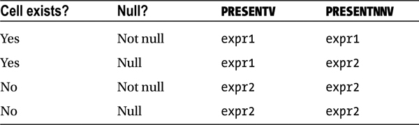
If the first argument cell_reference references an existing cell and if that cell contains a nonnull value, then the first argument, expr1, is returned; otherwise, the second argument, expr2, is returned. In contrast, the PRESENTV function checks for just the existence of a cell, whereas the PRESENTNNV function checks for both the existence of a cell and null values in that cell. Table 9-1 shows the values returned from these two functions in four different cases.
Table 9-1. PRESENTV and PRESENTNNV Comparison
You can define a lookup table and refer to that lookup table in the rules section. Such a lookup table is sometimes termed a reference table. Reference tables are defined in the initial section of the SQL statement and are then referred to in the rules section of the SQL statement.
In Listing 9-19, lines 5 through 9 define a lookup table ref_prod using a REFERENCE clause. Line 5 REFERENCE ref_prod is specifying ref_prod as a lookup table. Column prod_name is a dimension column as specified in line 8, and column prod_list_price is a measures column. Note that the reference table must be unique on the dimension column and should retrieve exactly one row per dimension column value.
Listing 9-19. Reference Model
 1     select year, week,sale, prod_list_price
 2        from sales_fact
 3        where country in ('Australia') and product ='Xtend Memory'
 4        model return updated rows
 5        REFERENCE ref_prod on
 6          (select prod_name, max(prod_list_price) prod_list_price
 7             from products group by prod_name)
 8           dimension by (prod_name)
 9           measures (prod_list_price)
10        MAIN main_section
11          partition by (product, country)
12          dimension by (year, week)
13          measures ( sale, receipts, 0 prod_list_price )
14          rules   (
15              prod_list_price[year,week] order by year, week =
16                                 ref_prod.prod_list_price [ cv(product) ]
17        )
18*   order by year, week;

 YEAR WEEK       SALE PROD_LIST_PRICE
----- ---- ---------- ---------------
 2000   31      44.78           20.99
 2000   33     134.11           20.99
 2000   34     178.52           20.99
...
Line 10 specifies the main model section starting with the keyword MAIN. This section is named main_section for ease of understanding, although any name can be used. In line 15, a rule for the column prod_list_price is specified and populated from the lookup table ref_prod. Line 16 shows that the reference table that measures columns is accessed using the clause ref_prod.prod_list_price [cv(product)]. The current value of the product column is passed as a lookup key in the lookup table using the clause cv(product).
In summary, you define a lookup table using a REFERENCE clause and then access that lookup table using the syntax look_table_name.measures column. For example, the syntax in this example is ref_prod.prod_list_price [cv(product)]. To access a specific row in the lookup table, you pass the current value of the dimension column from the left-hand side of the rule—in this example, using the cv(product) clause. You might be able to understand better if you imagine ref_prod as a table, cv(product) as the primary key for that table, and prod_list_price as a column to fetch from that lookup table.
More lookup tables can be added if needed. Suppose you also need to retrieve the country_iso_code column values from another table. You achieve this by adding the lookup table ref_country, as shown in Listing 9-20, lines 10 through 13. Column country_name is the dimension column and country_iso_code is a measures column. Lines 22 and 23 refer to the lookup table using a new rule Iso_code. This rule accesses the lookup table ref_country using the cv of the country column as the lookup key.
Listing 9-20. More Lookup Tables
 1     select year, week,sale,  prod_list_price, iso_code
 2        from sales_fact
 3        where country in ('Australia') and product ='Xtend Memory'
 4        model return updated rows
 5        REFERENCE ref_prod on
 6          (select prod_name, max(prod_list_price) prod_list_price from
 7             products group by prod_name)
 8           dimension by (prod_name)
 9           measures (prod_list_price)
10        REFERENCE ref_country on
11          (select country_name, country_iso_code from countries)
12           dimension by (country_name )
13           measures (country_iso_code)
14        MAIN main_section
15          partition by (product, country)
16          dimension by (year, week)
17          measures (  sale, receipts, 0 prod_list_price ,
18                              cast(' ' as varchar2(5)) iso_code)
19          rules   (
20              prod_list_price[year,week] order by year, week =
21                             ref_prod.prod_list_price [ cv(product) ],
22              iso_code [year, week] order by year, week =
23                             ref_country.country_iso_code [ cv(country)]
24        )
25*   order by year, week

YEAR WEEK       SALE PROD_LIST_PRICE ISO_C
---- ---- ---------- --------------- -----
2000   31      44.78           20.99 AU
2000   33     134.11           20.99 AU
2000   34     178.52           20.99 AU
2000   35      78.82           20.99 AU
2000   36     118.41           20.99 AU
 ...
In SQL statements using Model SQL, values can be null for two reasons: null values in the existing cells and references to nonexistent cells. I discuss the latter scenario in this section.
By default, the reference to nonexistent cells returns null values. In Listing 9-21, the rule in line 10 accesses the sale column for the year equal to 2002 and the week equal to 1 using the clause sale[2002,1]. There are no data in the sales_fact table for the year 2002, and so sale[2002,1] is accessing a nonexistent cell. Output in this listing is null because of the arithmetic operation with a null value.
Listing 9-21. KEEP NAV Example
  1    select product, country, year, week,  sale
  2    from sales_fact
  3    where country in ('Australia') and product ='Xtend Memory'
  4    model KEEP NAV return updated rows
  5    partition by (product, country)
  6    dimension by (year, week)
  7    measures ( sale)
  8    rules sequential  order(
  9      sale[2001,1] order by year, week= sale[2001,1],
 10      sale [ 2002, 1] order by year, week = sale[2001,1] + sale[2002,1]
 11      )
 12*   order by product, country,year, week

PRODUCT                        COUNTRY     YEAR WEEK       SALE
------------------------------ ---------- ----- ---- ----------
Xtend Memory                   Australia   2001    1      92.26
Xtend Memory                   Australia   2002    1
In line 4, I added a KEEP NAV clause after the MODEL keyword explicitly even though KEEP NAV is the default value. NAV stands for nonavailable values, and references to a nonexistent cell returns a null value by default.
This default behavior can be modified using the IGNORE NAV clause. Listing 9-22 shows an example. If the nonexistent cells are accessed, then 0 is returned for numeric columns and an empty string is returned for text columns instead of null values. You can see that the output in Listing 9-22 shows that a value of 92.26 is returned for the clause sale[2001,1] + sale[2002,1] and a 0 is retuned for the nonexisting cell sale[2002,1].
Listing 9-22. IGNORE NAV
  1    select product, country, year, week,  sale
  2    from sales_fact
  3    where country in ('Australia') and product ='Xtend Memory'
  4    model IGNORE NAV return updated rows
  5    partition by (product, country)
  6    dimension by (year, week)
  7    measures ( sale)
  8    rules sequential  order(
  9      sale[2001,1] order by year, week= sale[2001,1],
 10      sale [ 2002, 1] order by year, week = sale[2001,1] + sale[2002,1]
 11      )
 12*   order by product, country,year, week

PRODUCT                        COUNTRY     YEAR WEEK       SALE
------------------------------ ---------- ----- ---- ----------
Xtend Memory                   Australia   2001    1      92.26
Xtend Memory                   Australia   2002    1      92.26
The functions PRESENTV and PRESNTNNV are also useful in handling NULL values. Refer to the earlier section “Iteration” for a discussion and examples of these two functions.
Performance Tuning with the MODEL Clause
As with all SQL, sometimes you need to tune statements using the MODEL clause. To this end, it helps to know how to read execution plans involving the clause. It also helps to know about some of the issues you may encounter—such as predicate pushing and partitioning—when working with MODEL clause queries.
In the MODEL clause, rule evaluation is the critical step. Rule evaluation can use one of five algorithm types: ACYCLIC, ACYCLIC FAST, CYCLIC, ORDERED, and ORDERED FAST. The algorithm chosen depends on the complexity and dependency of the rules themselves. The algorithm chosen also affects the performance of the SQL statement. But, details of these algorithms are not well documented.
ACYCLIC FAST and ORDERED FAST algorithms are more optimized algorithms that allow cells to be evaluated efficiently. However, the algorithm chosen depends on the type of the rules that you specify. For example, if there is a possibility of a cycle in the rules, then the algorithm that can handle cyclic rules is chosen.
The algorithms of type ACYCLIC and CYCLIC are used if the SQL statement specifies the rules automatic order clause. An ORDERED type of the rule evaluation algorithm is used if the SQL statement specifies rules sequential order. If a rule accesses individual cells without any aggregation, then either the ACYCIC FAST or ORDERED FAST algorithm is used.
ACYCLIC
In Listing 9-23, a MODEL SQL statement and its execution plan is shown. Step 2 in the execution plan shows that this SQL is using the SQL MODEL ACYCLIC algorithm for rule evaluation. The keyword ACYCLIC indicates there are no possible cyclic dependencies between the rules. In this example, with the order by year, week clause you control the dependency between the rules, avoiding cycle dependencies,
Listing 9-23. Automatic order and ACYCLIC
  1    select product, country, year, week, inventory, sale, receipts
  2    from sales_fact
  3    where country in ('Australia') and product='Xtend Memory'
  4    model return updated rows
  5    partition by (product, country)
  6    dimension by (year, week)
  7    measures ( 0 inventory , sale, receipts)
  8    rules automatic order(
  9         inventory [year, week ] order by year, week  =
 10                    nvl(inventory [cv(year), cv(week)-1 ] ,0)
 11                  - sale[cv(year), cv(week) ] +
 12                  + receipts [cv(year), cv(week) ]
 13     )
 14*    order by product, country,year, week

---------------------------------------------------
| Id  | Operation           | Name       | E-Rows |
----------------------------------------------------
|   0 | SELECT STATEMENT    |            |        |
|   1 |  SORT ORDER BY      |            |    147 |
|   2 |   SQL MODEL ACYCLIC |            |    147 |
|*  3 |    TABLE ACCESS FULL| SALES_FACT |    147 |
---------------------------------------------------
ACYCLIC FAST
If a rule is a simple rule accessing just one cell, the ACYCLIC FAST algorithm can be used. The execution plan in Listing 9-24 shows that the ACYCLIC FAST algorithm is used to evaluate the rule in this example.
Listing 9-24. Automatic Order and ACYCLIC FAST
  1    select distinct product, country, year,week, sale_first_Week
  2    from sales_fact
  3    where country in ('Australia') and product='Xtend Memory'
  4    model return updated rows
  5    partition by (product, country)
  6    dimension by (year,week)
  7    measures ( 0 sale_first_week     ,sale )
  8    rules automatic order(
  9       sale_first_week [2000,1] = 0.12*sale [2000, 1]
 10     )
 11*    order by product, country,year, week

----------------------------------------------
| Id  | Operation               | Name       |
----------------------------------------------
|   0 | SELECT STATEMENT        |            |
|   1 |  SORT ORDER BY          |            |
|   2 |   SQL MODEL ACYCLIC FAST|            |
|*  3 |    TABLE ACCESS FULL    | SALES_FACT |
----------------------------------------------
CYCLIC
The execution plan in Listing 9-25 shows the use of the CYCLIC algorithm to evaluate the rules. The SQL in Listing 9-25 is a copy of Listing 9-23, except that the clause order by year, week is removed from the rule in line 9. Without the order by clause, row evaluation can happen in any order, and so the CYCLIC algorithm is chosen.
Listing 9-25. Automatic Order and CYCLIC
 1    select product, country, year, week, inventory, sale, receipts
 2    from sales_fact
 3    where country in ('Australia') and product='Xtend Memory'
 4    model return updated rows
 5    partition by (product, country)
 6    dimension by (year, week)
 7    measures ( 0 inventory , sale, receipts)
 8    rules automatic order(
 9         inventory [year, week ] =
10                    nvl(inventory [cv(year), cv(week)-1 ] ,0)
11                  - sale[cv(year), cv(week) ] +
12                  + receipts [cv(year), cv(week) ]
13     )
14*    order by product, country,year, week

------------------------------------------
| Id  | Operation           | Name       |
------------------------------------------
|   0 | SELECT STATEMENT    |            |
|   1 |  SORT ORDER BY      |            |
|   2 |   SQL MODEL CYCLIC  |            |
|*  3 |    TABLE ACCESS FULL| SALES_FACT |
------------------------------------------
Sequential
If the rule specifies sequential order, then the evaluation algorithm of the rules is shown as ORDERED. Listing 9-26 shows an example.
Listing 9-26. Sequential Order
 1    select product, country, year, week, inventory, sale, receipts
 2    from sales_fact
 3    where country in ('Australia') and product='Xtend Memory'
 4    model return updated rows
 5    partition by (product, country)
 6    dimension by (year, week)
 7    measures ( 0 inventory , sale, receipts)
 8    rules sequential order(
 9         inventory [year, week ] order by year, week =
10                    nvl(inventory [cv(year), cv(week)-1 ] ,0)
11                  - sale[cv(year), cv(week) ] +
12                  + receipts [cv(year), cv(week) ]
13     )
14*    order by product, country,year, week

-------------------------------------------
| Id  | Operation           | Name       |
-------------------------------------------
|   0 | SELECT STATEMENT    |            |
|   1 |  SORT ORDER BY      |            |
|   2 |   SQL MODEL ORDERED |            |
|*  3 |    TABLE ACCESS FULL| SALES_FACT |
-------------------------------------------
In a nutshell, the complexity and interdependency of the rules plays a critical role in the algorithm chosen. ACYCLIC FAST and ORDERED FAST algorithms are more scalable. This becomes important as the amount of data increases.
Conceptually, the Model clause is a variant of analytic SQL and is typically implemented in a view or inline view. Predicates are specified outside the view, and these predicates must be pushed into the view for acceptable performance. In fact, predicate pushing is critical to the performance of the Model clause. Unfortunately, not all predicates can be pushed safely into the view because of the unique nature of the Model clause. If predicates are not pushed, then the Model clause executes on the larger set of rows, which can result in poor performance.
In Listing 9-27, an inline view is defined from lines 2 through 14, and then predicates on columns country and product are added. Step 4 in the execution plan shows that both predicates are pushed into the view, rows are filtered applying these two predicates, and then the Model clause executes on the result set. This is good, because the Model clause is operating on a smaller set of rows than it would otherwise—just 147 rows in this case.
Listing 9-27. Predicate Pushing
  1   select * from (
  2    select product, country, year, week, inventory, sale, receipts
  3    from sales_fact
  4    model return updated rows
  5    partition by (product, country)
  6    dimension by (year, week)
  7    measures ( 0 inventory , sale, receipts)
  8    rules automatic order(
  9         inventory [year, week ] =
 10                    nvl(inventory [cv(year), cv(week)-1 ] ,0)
 11                  - sale[cv(year), cv(week) ] +
 12                  + receipts [cv(year), cv(week) ]
 13     )
 14   ) where country in ('Australia') and product='Xtend Memory'
 15*   order by product, country,year, week
...

select * from table (dbms_xplan.display_cursor('','','ALLSTATS LAST'));
-----------------------------------------------------------------------------
| Id  | Operation            | Name      | E-Rows|  OMem |  1Mem | Used-Mem |
-----------------------------------------------------------------------------
|   0 | SELECT STATEMENT     |           |       |       |       |          |
|   1 |  SORT ORDER BY       |           |    147| 18432 | 18432 |16384  (0)|
|   2 |   VIEW               |           |    147|       |       |          |
|   3 |    SQL MODEL CYCLIC  |           |    147|   727K|   727K|  358K (0)|
|*  4 |     TABLE ACCESS FULL| SALES_FACT|    147|       |       |          |
-----------------------------------------------------------------------------
Predicate Information (identified by operation id):
---------------------------------------------------
   4 - filter(("PRODUCT"='Xtend Memory' AND "COUNTRY"='Australia'))
Listing 9-28 is an example in which the predicates are not pushed into the view. In this example, predicate year=2000 is specified, but it is not pushed into the inline view. The optimizer estimates show that the MODEL clause needs to operate on some 111,000 rows.
Predicates can be pushed into a view only if it’s safe to do so. The SQL in Listing 9-28 uses both the year and week columns as dimension columns. In general, predicates on the partitioning columns can be pushed into a view safely, but not all predicates on the dimension column can be pushed.
Listing 9-28. Predicate Not Pushed
  1   select * from (
  2    select product, country, year, week, inventory, sale, receipts
  3    from sales_fact
  4    mod el return updated rows
  5    partition by (product, country)
  6    dimension by (year, week)
  7    measures ( 0 inventory , sale, receipts)
  8    rules automatic order(
  9         inventory [year, week ] =
 10                    nvl(inventory [cv(year), cv(week)-1 ] ,0)
 11                  - sale[cv(year), cv(week) ] +
 12                  + receipts [cv(year), cv(week) ]
 13     )
 14   ) where year=2000
 15*   order by product, country,year, week
-----------------------------------------------------------------------------
| Id  | Operation            | Name      | E-Rows|  OMem |  1Mem | Used-Mem |
-----------------------------------------------------------------------------
|   0 | SELECT STATEMENT     |           |       |       |       |          |
|   1 |  SORT ORDER BY       |           |   111K|  2604K|   733K| 2314K (0)|
|*  2 |   VIEW               |           |   111K|       |       |          |
|   3 |    SQL MODEL CYCLIC  |           |   111K|    12M|  1886K|   12M (0)|
|   4 |     TABLE ACCESS FULL| SALES_FACT|   111K|       |       |          |
-----------------------------------------------------------------------------

Predicate Information (identified by operation id):
---------------------------------------------------
   2 - filter("YEAR"=2000)
Typically, SQL statements using the MODEL clause access very large tables. Oracle’s query rewrite feature and materialized views can be combined to improve performance of such statements.
In Listing 9-29, a materialized view mv_model_inventory is created with the enable query rewrite clause. Subsequent SQL in the listing executes the SQL statement accessing the sales_fact table with the MODEL clause. The execution plan for the statement shows that the query rewrite feature rewrites the query, redirecting access to the materialized view instead of the base table. The rewrite improves the performance of the SQL statement because the materialized view has preevaluated the rules and stored the results.
![]() Note The fast incremental refresh is not available for materialized views involving the Model clause.
Note The fast incremental refresh is not available for materialized views involving the Model clause.
Listing 9-29. Materialized View and Query Rewrite
create materialized view mv_model_inventory
enable query rewrite as
  select product, country, year, week, inventory, sale, receipts
  from sales_fact
  model return updated rows
  partition by (product, country)
  dimension by (year, week)
  measures ( 0 inventory , sale, receipts)
  rules sequential order(
       inventory [year, week ] order by year, week =
                  nvl(inventory [cv(year), cv(week)-1 ] ,0)
                - sale[cv(year), cv(week) ] +
                + receipts [cv(year), cv(week) ]
   )
/
Materialized view created.

select * from (
 select product, country, year, week, inventory, sale, receipts
  from sales_fact
  model return updated rows
  partition by (product, country)
  dimension by (year, week)
  measures ( 0 inventory , sale, receipts)
  rules sequential order(
       inventory [year, week ] order by year, week =
                  nvl(inventory [cv(year), cv(week)-1 ] ,0)
                - sale[cv(year), cv(week) ] +
                + receipts [cv(year), cv(week) ]
   )
 )
where country in ('Australia') and product='Xtend Memory'
order by product, country,year, week
/

------------------------------------------------------------
| Id  | Operation                      | Name              |
------------------------------------------------------------
|   0 | SELECT STATEMENT               |                   |
|   1 |  SORT ORDER BY                 |                   |
|*  2 |   MAT_VIEW REWRITE ACCESS FULL | MV_MODEL_INVENTORY|
------------------------------------------------------------

Predicate Information (identified by operation id):
---------------------------------------------------
  2 - filter(("MV_MODEL_INVENTORY"."COUNTRY"='Australia' AND
             "MV_MODEL_INVENTORY"."PRODUCT"='Xtend Memory'))
MODEL -based SQL works seamlessly with Oracle’s parallel execution features. Queries against partitioned tables benefit greatly from parallelism and MODEL -based SQL statements.
An important concept with parallel query execution and MODEL SQL is that parallel query execution needs to respect the partition boundaries. Rules defined in the MODEL clause-based SQL statement might access another row. After all, accessing another row is the primary reason to use MODEL SQL statements. So, a parallel query slave must receive all rows from a model data partition so that the rules can be evaluated. This distribution of rows to parallel query slaves is taken care of seamlessly by the database engine. The first set of parallel slaves reads row pieces from the table and distributes the row pieces to a second set of slaves. The distribution is such that one slave receives all rows of a given model partition.
Listing 9-30 shows an example of MODEL and parallel queries. Two sets of parallel slaves are allocated to execute the statement shown. The first set of slaves is read from the table; the second set of slaves evaluates the MODEL rule.
Listing 9-30. Model and Parallel Queries
select  /*+ parallel ( sf 4) */
  product, country, year, week, inventory, sale, receipts
  from sales_fact sf
  where country in ('Australia') and product='Xtend Memory'
  model return updated rows
  partition by (product, country)
  dimension by (year, week)
  measures ( 0 inventory , sale, receipts)
  rules automatic order(
       inventory [year, week ] order by year, week =
                  nvl(inventory [cv(year), cv(week)-1 ] ,0)
                - sale[cv(year), cv(week) ] +
                + receipts [cv(year), cv(week) ]
   )
/
-----------------------------------------------...--------------------------
| Id  | Operation                | Name       |    TQ  |IN-OUT| PQ Distrib |
----------------------------------------------------------------------------
|   0 | SELECT STATEMENT         |            |...     |      |            |
|   1 |  PX COORDINATOR          |            |        |      |            |
|   2 |   PX SEND QC (RANDOM)    | :TQ10001   |  Q1,01 | P->S | QC (RAND)  |
|   3 |    BUFFER SORT           |            |  Q1,01 | PCWP |            |
|   4 |     SQL MODEL ACYCLIC    |            |  Q1,01 | PCWP |            |
|   5 |      PX RECEIVE          |            |  Q1,01 | PCWP |            |
|   6 |       PX SEND HASH       | :TQ10000   |  Q1,00 | P->P | HASH       |
|   7 |        PX BLOCK ITERATOR |            |  Q1,00 | PCWC |            |
|*  8 |         TABLE ACCESS FULL| SALES_FACT |  Q1,00 | PCWP |            |
----------------------------------------------------------------------------
Predicate Information (identified by operation id):
---------------------------------------------------
   8 - access(:Z>=:Z AND :Z<=:Z)
       filter(("PRODUCT"='Xtend Memory' AND "COUNTRY"='Australia'))
Partitioning in MODEL Clause Execution
Table partitioning can be used to improve the performance of MODEL SQL statements. In general, if the partitioning columns in the MODEL SQL matches the partitioning keys of the table, partitions are pruned. Partition pruning is a technique for performance improvement to limit scanning few partitions.
In Listing 9-31, the table sales_fact_part is list partitioned by year using the script Listing_9_31_partition.sql (part of the example download for this book). The partition with partition_id=3 contains rows with the value of 2000 for the year column. Because the MODEL SQL is using year as the partitioning column and because a year=2000 predicate is specified, partition pruning lead to scanning partition 3 alone. The execution plan shows that both the pstart and pstop columns have a value of 3, indicating that the range of partitions to be processed begins and ends with the single partition having an ID equal to 3.
Listing 9-31. Partition Pruning
select * from (
  select product, country, year, week, inventory, sale, receipts
  from sales_fact_part sf
  model return updated rows
  partition by (year, country )
  dimension by (product, week)
  measures ( 0 inventory , sale, receipts )
  rules automatic order(
       inventory [product, week ] order by product,  week =
                  nvl(inventory [cv(product),  cv(week)-1 ] ,0)
                - sale[cv(product),  cv(week) ] +
                + receipts [cv(product), cv(week) ]
   )
 )   where year=2000 and country='Australia' and product='Xtend Memory'
/
--------------------------------------------------...----------------
| Id  | Operation              | Name            |... Pstart| Pstop |
---------------------------------------------------------------------
|   0 | SELECT STATEMENT       |                 |          |       |
|   1 |  SQL MODEL ACYCLIC     |                 |          |       |
|   2 |   PARTITION LIST SINGLE|                 |      KEY |   KEY |
|*  3 |    TABLE ACCESS FULL   | SALES_FACT_PART |        3 |     3 |
---------------------------------------------------------------------

Predicate Information (identified by operation id):
---------------------------------------------------
   1 - filter("PRODUCT"='Xtend Memory')
   4 - filter("COUNTRY"='Australia')
In Listing 9-32, columns product and county are used as partitioning columns, but the table sales_fact_part has the year column as the partitioning key. Step 1 in the execution plan indicates that predicate year=2000 was not pushed into the view because the rule can access other partitions (because year is a dimension column). Because the partitioning key is not pushed into the view, partition pruning is not allowed and all partitions are scanned. You can see that pstart and pstop are 1 and 5, respectively, in the execution plan.
Listing 9-32. No Partition Pruning
  select * from (
  select product, country, year, week, inventory, sale, receipts
  from sales_fact_part sf
  model return updated rows
  partition by (product, country)
  dimension by (year, week)
  measures ( 0 inventory , sale, receipts)
  rules automatic order(
       inventory [year, week ] order by year,  week =
                  nvl(inventory [cv(year),  cv(week)-1 ] ,0)
                - sale[cv(year),  cv(week) ] +
                + receipts [cv(year), cv(week) ]
   )
 )   where year=2000 and country='Australia' and product='Xtend Memory'
/
------------------------------------------------...-------------
| Id  | Operation            | Name            | Pstart| Pstop |
----------------------------------------------------------------
|   0 | SELECT STATEMENT     |                 |       |       |
|*  1 |  VIEW                |                 |       |       |
|   2 |   SQL MODEL ACYCLIC  |                 |       |       |
|   3 |    PARTITION LIST ALL|                 |     1 |     5 |
|*  4 |     TABLE ACCESS FULL| SALES_FACT_PART |     1 |     5 |
------------------------------------------------...-------------
Predicate Information (identified by operation id):
---------------------------------------------------
 1 - filter("YEAR"=2000)
 4 - filter(("PRODUCT"='Xtend Memory' AND "COUNTRY"='Australia'))
Indexes
Choosing indexes to improve the performance of SQL statements using a MODEL clause is no different from choosing indexes for any other SQL statements. You use the access and filter predicates to determine the optimal indexing strategy.
As an example, the execution plan in Listing 9-32 shows that the filter predicates "PRODUCT"='Xtend Memory' and "COUNTRY"='Australia' are applied at step 4. Indexing on the two columns product and country is helpful if there are many executions with these column predicates.
In Listing 9-33, I added an index to the columns country and product. The resulting execution plan shows table access via the index, possibly improving performance.
Listing 9-33. Indexing with SQL Access in Mind
  create index sales_fact_part_i1 on sales_fact_part (country, product) ;
  select * from (
  select product, country, year, week, inventory, sale, receipts
  from sales_fact_part sf
  model return updated rows
  partition by (product, country)
  dimension by (year, week)
  measures ( 0 inventory , sale, receipts)
  rules automatic order(
       inventory [year, week ] order by year,  week =
                  nvl(inventory [cv(year),  cv(week)-1 ] ,0)
                - sale[cv(year),  cv(week) ] +
                + receipts [cv(year), cv(week) ]
   )
 )   where year=2000 and country='Australia' and product='Xtend Memory'
/

-----------------------------------------------------------------------------
|Id |Operation                            |Name              | Pstart| Pstop|
-----------------------------------------------------------------------------
| 0 |SELECT STATEMENT                     |                  |       |      |
|*1 | VIEW                                |                  |       |      |
| 2 |  SQL MODEL ACYCLIC                  |                  |       |      |
| 3 |   TABLE ACCESS BY GLOBAL INDEX ROWID|SALES_FACT_PART   | ROWID | ROWID|
|*4 |    INDEX RANGE SCAN                 |SALES_FACT_PART_I1|       |      |
-----------------------------------------------------------------------------

Predicate Information (identified by operation id):r
---------------------------------------------------
   1 - filter("YEAR"=2000)
   4 - access("COUNTRY"='Australia' AND "PRODUCT"='Xtend Memory')
In a business setting, requirements are complex and multiple levels of aggregation are often needed. When writing complex queries, you can often combine subquery factoring with the MODEL clause to prevent a SQL statement from becoming unmanageably complex.
Listing 9-34 provides one such example. Two MODEL clauses are coded in the same SQL statement. The first MODEL clause is embedded within a view that is the result of a subquery being factored into the WITH clause. The main query uses that view to pivot the value of the sale column from the prior year. The output shows that the prior week’s sales are pivoted into the current week’s row.
Listing 9-34. More Indexing with SQL Access in Mind
with t1 as (
  select  product, country, year, week, inventory, sale, receipts
  from sales_fact sf
  where country in ('Australia') and product='Xtend Memory'
  model return updated rows
  partition by (product, country)
  dimension by (year, week)
  measures ( 0 inventory , sale, receipts)
  rules automatic order(
       inventory [year, week ] order by year, week =
                  nvl(inventory [cv(year), cv(week)-1 ] ,0)
                - sale[cv(year), cv(week) ] +
                + receipts [cv(year), cv(week) ]
   )
)
select product, country, year, week , inventory,
sale, receipts, prev_sale
from t1
model return updated rows
partition by (product, country)
dimension by (year, week)
measures (inventory, sale, receipts,0 prev_sale)
rules sequential order (
  prev_sale [ year, week ] order by year, week =
                nvl (sale [ cv(year) -1, cv(week)],0 )
)
order by 1,2,3,4
/

PRODUCT         COUNTRY     YEAR  WEEK    INVENTORY    SALE     RECEIPTS      PREV_SALE
--------------- ----------- ----- ----- ------------ -------- ----------- --------------
Xtend Memory      Australia  1998     1         8.88    58.15       67.03              0
...
Xtend Memory      Australia  1999     1        2.676    53.52      56.196          58.15
...
Xtend Memory      Australia  2000     1      -11.675    46.7       35.025          53.52
...
Xtend Memory      Australia  2001     1        4.634    92.26      96.894           46.7
Summary
I can’t stress enough the importance of thinking in terms of sets when writing SQL statements. Many SQL statements can be rewritten concisely using the MODEL clause discussed in this chapter. As an added bonus, rewritten queries such as model or analytic functions can perform much better than traditional SQL statements. A combination of subquery factoring, model, and analytic functions features can be used effectively to implement complex requirements.