
![]()
Indexes
Indexes are critical structures needed for efficient retrieval of rows, for uniqueness enforcement, and for the efficient implementation of referential constraints. Oracle Database provides many index types suited for different needs of application access methods. Effective choice of index type and critical choice of columns to index are of paramount importance for optimal performance. Inadequate or incorrect indexing strategy can lead to performance issues. In this chapter, I discuss basic implementation of indexes, various index types, their use cases, and strategy to choose optimal index type. Indexes available in Oracle Database as of version 12c can be classified broadly into one of three categories based on the algorithm they use: B-tree indexes, bitmap indexes, and index-organized tables, or IOTs.
Implementation of bitmap indexes is suitable for columns with infrequent update, insert, and delete activity. Bitmap indexes are better suited for static columns with lower distinct values—a typical case in data warehouse applications. A gender column in a table holding population data is a good example, because as there are only a few distinct values for this column. I discuss this in more detail later in this chapter.
![]() Note All tables mentioned in this chapter refer to the objects in SH schema supplied by Oracle Corporation example scripts.
Note All tables mentioned in this chapter refer to the objects in SH schema supplied by Oracle Corporation example scripts.
B-tree indexes are commonly used in all applications. There are many index types such as partitioned indexes, compressed indexes, and function-based indexes implemented as B-tree indexes. Special index types such as IOTs and secondary indexes on IOTs are also implemented as B-tree indexes.
THE IMPORTANCE OF CHOOSING CORRECTLY
I have a story to share about the importance of indexing choice. During an application upgrade, an application designer chose bitmap indexes on a few key tables that were modified heavily. After the application upgrade, the application response time was not acceptable. Because this application was a warehouse management application, performance issues were affecting the shipping and order fulfillment process of this U.S. retail giant.
We were called in to troubleshoot the issue. We reviewed the database performance metrics and quickly realized that the poor choice of index type was the root cause of the performance issue. Database metrics were showing that the application was suffering from locking contention, too. These bitmap indexes used to grow from about 100MB in the morning to around 4 to 5GB by midafternoon. The designer even introduced a job to rebuild the index at regular intervals. We resolved the issue by converting the bitmap indexes to B-tree indexes. This story demonstrates you the importance of choosing an optimal indexing strategy.
Understanding Indexes
Is a full table scan access path always bad? Not necessarily. Efficiency of an access path is very specific to the construction of the SQL statement, application data, distribution of data, and the environment. No one access path is suitable for all execution plans. In some cases, a full table scan access path is better than an index-based access path. Next, I discuss choice of index usage, considerations for choosing columns to index, and special considerations for null clauses.
When to Use Indexes
In general, index-based access paths perform better if the predicates specified in the SQL statement are selective—meaning, that few rows are fetched applying the specified predicates. A typical index-based access path usually involves following three steps:
- Traversing the index tree and collecting the rowids from the leaf block after applying the SQL predicates on indexed columns
- Fetching the rows from the table blocks using the rowids
- Applying the remainder of the predicates on the rows fetched to derive a final result set
The second step of accessing the table block is costlier if numerous rowids are returned during step 1. For every rowid from the index leaf blocks, table blocks need to be accessed, and this might result in multiple physical IOs, leading to performance issues. Furthermore, table blocks are accessed one block at a time physically and can magnify performance issues. For example, consider the SQL statement in Listing 12-1 accessing the sales table with just one predicate, country= 'Spain'; the number of rows returned from step 5 is estimated to be 7985. So, 7985 rowids estimated to be retrieved from that execution step and table blocks must be accessed at least 7985 times to retrieve the row pieces. Some of these table block accesses might result in physical IO if the block is not in the buffer cache already. So, the index-based access path might perform worse for this specific case.
Listing 12-1. Index Access Path
create index sales_fact_c2 on sales_fact ( country);

select /*+ index (s sales_fact_c2) */ count(distinct(region))
from sales_fact s where country='Spain';

--------------------------------------------------------------------------
| Id  | Operation                  | Name          | E-Rows | Cost (%CPU)|
--------------------------------------------------------------------------
|   0 | SELECT STATEMENT           |               |        |   930 (100)|
|   1 |  SORT AGGREGATE            |               |      1 |            |
|   2 |   VIEW                     | VW_DAG_0      |      7 |   930   (0)|
|   3 |    HASH GROUP BY           |               |      7 |   930   (0)|
|   4 |     TABLE ACCESS BY INDEX  | SALES_FACT    |   7985 |   930   (0)|
|     |           ROWID BATCHED    |               |        |            |
|*  5 |      INDEX RANGE SCAN      | SALES_FACT_C2 |   7985 |    26   (0)|
--------------------------------------------------------------------------

select count(distinct(region)) from sales_fact s where country='Spain';

-----------------------------------------------------------------
| Id  | Operation            | Name       | E-Rows | Cost (%CPU)|
-----------------------------------------------------------------
|   0 | SELECT STATEMENT     |            |        |   309 (100)|
|   1 |  SORT AGGREGATE      |            |      1 |            |
|   2 |   VIEW               | VW_DAG_0   |      7 |   309   (1)|
|   3 |    HASH GROUP BY     |            |      7 |   309   (1)|
|*  4 |     TABLE ACCESS FULL| SALES_FACT |   7985 |   309   (1)|
-----------------------------------------------------------------
In Listing 12-1, in the first SELECT statement, I force an index-based access path using the hint index (s sales_fact_c2), and the optimizer estimates the cost of the index-based access plan as 930. The execution plan for the next SELECT statement without the hint shows that the optimizer estimates the cost of the full table scan access path as 309. Evidently, the full table scan access path is estimated to be cheaper and more suited for this SQL statement.
![]() Note In Listing 12-1 and the other listings in this chapter, the statements have been run and their execution plans displayed. However, for brevity, much of the output has been elided.
Note In Listing 12-1 and the other listings in this chapter, the statements have been run and their execution plans displayed. However, for brevity, much of the output has been elided.
Let’s consider another SELECT statement. In Listing 12-2, all three columns are specified in the predicate of the SQL statement. Because the predicates are more selective, the optimizer estimates that eight rows will be retrieved from this SELECT statement, and the cost of the execution plan is 3. I force the full table scan execution plan in the subsequent SELECT statement execution, and then the cost of this execution plan is 309. Index-based access is more optimal for this SQL statement.
Listing 12-2. Index Access Path 2
select product, year, week from sales_fact
where product='Xtend Memory' and  year=1998 and week=1;

----------------------------------------------------------------
| Id  | Operation        | Name          | E-Rows | Cost (%CPU)|
----------------------------------------------------------------
|   0 | SELECT STATEMENT |               |        |     3 (100)|
|*  1 |  INDEX RANGE SCAN| SALES_FACT_C1 |      8 |     3   (0)|
----------------------------------------------------------------

select /*+ full(sales_fact) */ product, year, week from sales_fact where product='Xtend Memory'and year=1998 and week=1;

--------------------------------------------------------------
| Id  | Operation         | Name       | E-Rows | Cost (%CPU)|
--------------------------------------------------------------
|   0 | SELECT STATEMENT  |            |        |   309 (100)|
|*  1 |  TABLE ACCESS FULL| SALES_FACT |      8 |   309   (1)|
--------------------------------------------------------------
Evidently, no single execution plan is better for all SQL statements. Even for the same statement, depending on the data distribution and the underlying hardware, execution plans can behave differently. If the data distribution changes, the execution plans can have different costs. This is precisely why you need to collect statistics that reflect the distribution of data so the optimizer can choose the optimal plan.
Furthermore, full table scans and fast full scans perform multiblock read calls whereas index range scans or index unique scans do single-block reads. Multiblock reads are much more efficient than single-block reads on a block-by-block basis. Optimizer calculations factor this difference and choose an index-based access path or full table access path as appropriate. In general, an Online Transaction Processing (OLTP) application uses index-based access paths predominantly, and the data warehouse application uses full table access paths predominantly.
A final consideration is parallelism. Queries can be tuned to execute faster using parallelism when the predicates are not selective enough. The cost of an execution plan using a parallel full table scan can be cheaper than the cost of a serial index range scan, leading to an optimizer choice of a parallel execution plan.
Choosing optimal columns for indexing is essential to improve SQL access performance. The choice of columns to index should match the predicates used by the SQL statements. The following are considerations for choosing an optimal indexing column:
- If the application code uses the equality or range predicates on a column while accessing a table, it’s a good strategy to consider indexing that column. For multicolumn indexes, the leading column should be the column used in most predicates. For example, if you have a choice to index the columns c1 and c2, then the leading column should be the column used in most predicates.
- It is also important to consider the cardinality of the predicates and the selectivity of the columns. For example, if a column has just two distinct values with a uniform distribution, then that column is probably not a good candidate for B-tree indexes because 50 percent of the rows will be fetched by equality predicates on the column value. On the other hand, if the column has two distinct values with skewed distribution—in other words, one value occurs in a few rows and the application accesses that table with the infrequently occurring column value—it is preferable to index that column.
- An example is a processed column in a work-in-progress table with three distinct values (P, N, and E). The application accesses that table with the processed=‘N’ predicate. Only a few unprocessed rows are left with a status of ‘N’ in processed_column, so access through the index is optimal. However, queries with the predicate Processed=‘Y’ should not use the index because nearly all rows are fetched by this predicate. Histograms can be used so that the optimizer can choose the optimal execution plan, depending on the literal or bind variables.
![]() Note Cardinality is defined as the number of rows expected to be fetched by a predicate or execution step. Consider a simple equality predicate on the column assuming uniform distribution in the column values. Cardinality is calculated as the number of rows in the table divided by the number of distinct values in the column. For example, in the sales table, there are 918,000 rows in the table, and the prod_id column has 72 distinct values, so the cardinality of the equality predicate on the prod_id column is 918,000 ÷ 72 = 12,750. So, in other words, the predicate prod_id=:b1 expects to fetch 12,750 rows. Columns with lower cardinality are better candidates for indexing because the index selectivity is better. For unique columns, cardinality of an equality predicate is one. Selectivity is a measure ranging between zero and one, simplistically defined as 1 ÷ NDV, where NDV stands for number of distinct values. So, the cardinality of a predicate can be defined as the selectivity multiplied by the number of rows in the table.
Note Cardinality is defined as the number of rows expected to be fetched by a predicate or execution step. Consider a simple equality predicate on the column assuming uniform distribution in the column values. Cardinality is calculated as the number of rows in the table divided by the number of distinct values in the column. For example, in the sales table, there are 918,000 rows in the table, and the prod_id column has 72 distinct values, so the cardinality of the equality predicate on the prod_id column is 918,000 ÷ 72 = 12,750. So, in other words, the predicate prod_id=:b1 expects to fetch 12,750 rows. Columns with lower cardinality are better candidates for indexing because the index selectivity is better. For unique columns, cardinality of an equality predicate is one. Selectivity is a measure ranging between zero and one, simplistically defined as 1 ÷ NDV, where NDV stands for number of distinct values. So, the cardinality of a predicate can be defined as the selectivity multiplied by the number of rows in the table.
- Think about column ordering, and arrange the column order in the index to suit the application access patterns. For example, in the sales table, the selectivity of the prod_id column is 1 ÷ 72 and the selectivity of the cust_id column is 1 ÷ 7059. It might appear that column cust_id is a better candidate for indexes because the selectivity of that column is lower. However, if the application specifies equality predicates on the prod_id column and does not specify cust_id column in the predicate, then the cust_id column need not be indexed even though the cust_id column has better selectivity. If the application uses the predicates on both the prod_id and cust_id columns, then it is preferable to index both columns, with the cust_id column as the leading column. Consideration should be given to the column usage in the predicates instead of relying on the selectivity of the columns.
- You should also consider the cost of an index. Inserts, deletes, and updates (updating the indexed columns) maintain the indexes—meaning, if a row is inserted into the sales table, then a new value pair is added to the index matching the new value. This index maintenance is costlier if the columns are updated heavily, because the indexed column update results in a delete and insert at the index level internally, which could introduce additional contention points, too.
- Consider the length of the column. If the indexed column is long, then the index is big. The cost of that index may be higher than the overall gain from the index. A bigger index also increases undo size and redo size.
- In a multicolumn index, if the leading column has only a few distinct values, consider creating that index as a compressed index. The size of these indexes are then smaller, because repeating values are not stored in a compressed index. I discuss compressed indexes later in this chapter.
- If the predicates use functions on indexed columns, the index on that column may not be chosen. For example, the predicate to_char(prod_id) =:B1 applies a to_char function on the prod_id column. A conventional index on the prod_id column might not be chosen for this predicate, and a function-based index needs to be created on the to_char(prod_id) column.
- Do not create bitmap indexes on columns modified aggressively. Internal implementation of a bitmap index is more suitable for read-only columns with few distinct values. The size of the bitmap index grows rapidly if the indexed columns are updated. Excessive modification to a bitmap index can lead to enormous locking contention, too. Bitmap indexes are more prevalent in data warehouse applications.
The Null Issue
It is common practice for a SQL statement to specify the IS NULL predicate. Null values are not stored in single-column indexes, so the predicate IS NULL does not use a single-column index. But, null values are stored in a multicolumn index. By creating a multicolumn index with a dummy second column, you can enable the use of an index for the IS NULL clause
In Listing 12-3, a single-column index T1_N1 is created on column n1. The optimizer does not choose the index access path for the SELECT statement with the predicate n1 is null. Another index, t1_n10, is created on the expression (n1,0), and the optimizer chooses the access path using the index because the null values are stored in this multicolumn index. The size of the index is kept smaller by adding a dummy value of 0 to the index.
Listing 12-3. NULL Handling
drop table t1;
create table  t1 (n1 number, n2 varchar2(100) );
insert into t1 select object_id, object_name from dba_objects where rownum<101;
commit;
create index t1_n1 on t1(n1);
select * from t1 where n1 is null;

--------------------------------------------------------
| Id  | Operation         | Name | E-Rows | Cost (%CPU)|
--------------------------------------------------------
|   0 | SELECT STATEMENT  |      |        |     3 (100)|
|*  1 |  TABLE ACCESS FULL| T1   |      1 |     3   (0)|
--------------------------------------------------------

create index t1_n10 on t1(n1,0);
select * from t1 where n1 is null;

----------------------------------------------------------------------------
| Id  | Operation                           | Name   | E-Rows | Cost (%CPU)|
----------------------------------------------------------------------------
|   0 | SELECT STATEMENT                    |        |        |     2 (100)|
|   1 |  TABLE ACCESS BY INDEX ROWID BATCHED| T1     |      1 |     2   (0)|
|*  2 |   INDEX RANGE SCAN                  | T1_N10 |      5 |     1   (0)|
----------------------------------------------------------------------------
Index Structural Types
Oracle Database provides various types of indexes to suit application access paths. These index types can be classified loosely into three broad categories based on the structure of an index: B-tree indexes, bitmap indexes, and IOTs.
B-tree indexes implement a structure similar to an inverted tree with a root node, branch nodes, and leaf nodes, and they use tree traversal algorithms to search for a column value. The leaf node holds the (value, rowid) pair for that index key column, and the rowid refers to the physical location of a row in the table block. The branch block holds the directory of leaf blocks and the value ranges stored in those leaf blocks. The root block holds the directory of branch blocks and the value ranges addressed in those branch blocks.
Figure 12-1 shows the B-tree index structure for a column with a number datatype. This figure is a generalization of the index structure to help you improve your understanding; the actual index structures are far more complex. The root block of the index holds branch block addresses and the range of values addressed in the branch blocks. The branch blocks hold the leaf block addresses and the range of values stored in the leaf blocks.
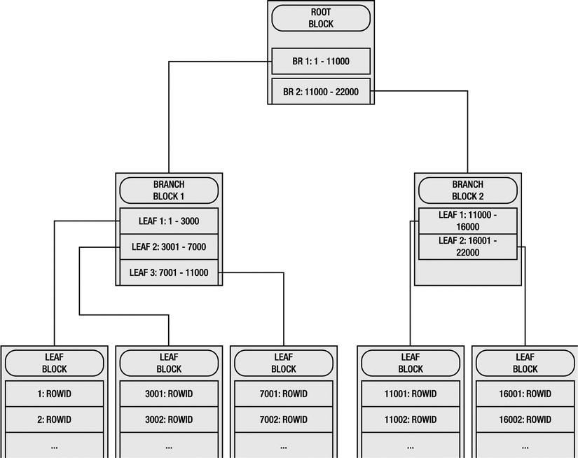
Figure 12-1. B-tree index structure
A search for a column value using an index usually results in an index range scan or an index unique scan. Such a search starts at the root block of the index tree, traverses to the branch block, and then traverses to the leaf block. Rowids are fetched from the leaf blocks from the (column value, rowid) pairs, and each row piece is fetched from the table block using the rowid. Without the indexes, searching for a key inevitably results in a full table scan of the table.
In Figure 12-1, if the SQL statement is searching for a column value of 12,000 with a predicate n1=12000, the index range scan starts at the root block, traverses to the second branch block because the second branch block holds the range of values from 11,001 to 22,000, and then traverses to the fourth leaf block because that leaf block holds the column value range from 11,001 to 16,000. As the index stores the sorted column values, the range scan quickly accesses the column value matching n1=12000 from the leaf block entries, reads the rowids associated with that column value, and accesses the rows from the table using those rowids. Rowids are pointers to the physical location of a row in the table block.
B-tree indexes are suitable for columns with lower selectivity. If the columns are not selective enough, the index range scan is slower. Furthermore, less selective columns retrieve numerous rowids from the leaf blocks, leading to excessive single-block access to the table.
Bitmap indexes are organized and implemented differently than B-tree indexes. Bitmaps are used to associate the rowids with the column value. Bitmap indexes are not suitable for columns with a higher number of updates or for tables with heavy Data Manipulation Language (DML)activity. Bitmap indexes are suitable for data warehouse tables with mostly read-only operations on columns with lower distinct values. If the tables are loaded regularly, as in the case of a typical data warehouse table, it is important to drop the bitmap index before the load, then load the data and recreate the bitmap index.
Bitmap indexes can be created on partitioned tables, too, but they must be created as local indexes. As of Oracle Database release 12c, bitmap indexes cannot be created as global indexes. Bitmap indexes cannot be created as unique indexes either.
In Listing 12-4, two new bitmap indexes are added on columns country and region. The SELECT statement specifies predicates on columns country and region. The execution plan shows three major operations: bitmaps from the bitmap index sales_fact_part_bm1 fetched by applying the predicate country=‘Spain’, bitmaps from the bitmap index sales_fact_part_bm2 fetched by applying the predicate region=‘Western Europe’, and then those two bitmaps are ANDed to calculate the final bitmap using the BITMAP AND operation.The resulting bitmap is converted to rowids, and the table rows are accessed using those rowids.
Listing 12-4. Bitmap Indexes
drop index sales_fact_part_bm1;
drop index sales_fact_part_bm2;

create bitmap index sales_fact_part_bm1 on sales_fact_part ( country ) Local;
create bitmap index sales_fact_part_bm2 on sales_fact_part ( region ) Local;

select * from sales_fact_part
where country='Spain' and region='Western Europe' ;

-----------------------------------------------------------------------------
| Id  | Operation                     | Name                | Pstart| Pstop |
-----------------------------------------------------------------------------
|   0 | SELECT STATEMENT              |                     |       |       |
|   1 |  PARTITION LIST ALL           |                     |     1 |     5 |
|   2 |   TABLE ACCESS BY LOCAL INDEX | SALES_FACT_PART     |     1 |     5 |
|     |         ROWID BATCHED         |                     |       |       |
|   3 |    BITMAP CONVERSION TO ROWIDS|                     |       |       |
|   4 |     BITMAP AND                |                     |       |       |
|*  5 |      BITMAP INDEX SINGLE VALUE| SALES_FACT_PART_BM1 |     1 |     5 |
|*  6 |      BITMAP INDEX SINGLE VALUE| SALES_FACT_PART_BM2 |     1 |     5 |
-----------------------------------------------------------------------------
Bitmap indexes can introduce severe locking issues if the index is created on columns modified heavily by DML activity. Updates to a column with a bitmap index must update a bitmap, and the bitmaps usually cover a set of rows. So, an update to one row can lock a set of rows in that bitmap. Bitmap indexes are used predominantly in data warehouse applications; they are of limited use in OLTP applications.
Conventional tables are organized as heap tables because the table rows can be stored in any table block. Fetching a row from a conventional table using a primary key involves primary key index traversal, followed by a table block access using the rowid. In IOTs, the table itself is organized as an index, all columns are stored in the index tree itself, and the access to a row using a primary key involves index access only. This access using IOTs is better because all columns can be fetched by accessing the index structure, thereby avoiding the table access. This is an efficient access pattern because the number of accesses is minimized.
With conventional tables, every row has a rowid. When rows are created in a conventional table, they do not move (row chaining and row migration are possible, but the headpiece of the row does not move). However, IOT rows are stored in the index structure itself, so rows can be migrated to different leaf blocks as a result of DML operations, resulting in index leaf block splitting and merging. In a nutshell, rows in the IOTs do not have physical rowids whereas rows in the heap tables always have fixed rowids.
IOTs are appropriate for tables with the following properties:
- Tables with shorter row length: Tables with fewer short columns are appropriate for IOTs. If the row length is longer, the size of the index structure can be unduly large, leading to more resource usage than the heap tables.
- Tables accessed mostly through primary key columns: Although secondary indexes can be created on IOTs, secondary indexes can be resource intensive if the primary key is longer. I cover secondary indexes later in this section.
In Listing 12-5, an IOT sales_iot is created by specifying the keywords organization index. Note that the SELECT statement specifies only a few columns in the primary key, and the execution plan shows that columns are retrieved by an index range scan, thereby avoiding a table access. Had this been a conventional heap table, you would see an index unique scan access path followed by rowid-based table access.
Listing 12-5. Index Organized Tables
drop table sales_iot;
create table sales_iot
  ( prod_id number not null,
    cust_id number not null,
    time_id date not null,
    channel_id number not null,
    promo_id number not null,
    quantity_sold number (10,2) not null,
    amount_sold number(10,2) not null,
    primary key  ( prod_id, cust_id, time_id, channel_id, promo_id)
 )
organization index ;
insert into sales_iot select * from sales;
commit;

@analyze_table

select quantity_sold, amount_sold from sales_iot where
prod_id=13 and cust_id=2 and channel_id=3 and promo_id=999;

--------------------------------------------------------------------
| Id  | Operation        | Name              | E-Rows | Cost (%CPU)|
--------------------------------------------------------------------
|   0 | SELECT STATEMENT |                   |        |     3 (100)|
|*  1 |  INDEX RANGE SCAN| SYS_IOT_TOP_94835 |      1 |     3   (0)|
--------------------------------------------------------------------
A secondary index can be created on an IOT, too. Conventional indexes store the (column value, rowid) pair. But, in IOTs, rows do not have a physical rowid; instead, a (column value, logical rowid) pair is stored in the secondary index. This logical rowid is essentially a primary key column with the values of the row stored efficiently. Access through the secondary index fetches the logical rowid using the secondary index, then uses the logical rowid to access the row piece using the primary key IOT structure.
In Listing 12-6, a secondary index sales_iot_sec is created on an IOT sales_iot. The SELECT statement specifies the predicates on secondary index columns. The execution plan shows an all index access, where logical rowids are fetched from the secondary index sales_iot_sec with an index range scan access method, and then rows are fetched from the IOT primary key using the logical rowids fetched with an index unique scan access method. Also, note that the size of the secondary index is nearly one half the size of the primary index, and secondary indexes can be resource intensive if the primary key is longer.
Listing 12-6. Secondary Indexes on an IOT
drop index sales_iot_sec ;
create index sales_iot_sec on
 sales_iot (channel_id, time_id, promo_id, cust_id) ;

select quantity_sold, amount_sold from sales_iot where
channel_id=3 and promo_id=999 and cust_id=12345 and time_id='30-JAN-00';

---------------------------------------------------------------------
| Id  | Operation         | Name              | E-Rows | Cost (%CPU)|
---------------------------------------------------------------------
|   0 | SELECT STATEMENT  |                   |        |     7 (100)|
|*  1 |  INDEX UNIQUE SCAN| SYS_IOT_TOP_94835 |      4 |     7   (0)|
|*  2 |   INDEX RANGE SCAN| SALES_IOT_SEC     |      4 |     3   (0)|
---------------------------------------------------------------------

select segment_name, sum( bytes/1024/1024) sz from dba_segments
where segment_name in ('SYS_IOT_TOP_94835','SALES_IOT_SEC')
group by segment_name ;

SEGMENT_NAME                           SZ
------------------------------ ----------
SALES_IOT_SEC                          36
SYS_IOT_TOP_94835                      72
IOTs are special structures that are useful to eliminate additional indexes on tables with short rows that undergo heavy DML and SELECT activity. However, adding secondary indexes on IOTs can cause an increase in index size, redo size, and undo size if the primary key is longer.
Partitioned Indexes
Indexes can be partitioned similar to a table partitioning scheme. There is a variety of ways to partition the indexes. Indexes can be created on partitioned tables as local or global indexes, too. Furthermore, there are various partitioning schemes available, such as range partitioning, hash partitioning, list partitioning, and composite partitioning. From Oracle Database version 10g onward, partitioned indexes also can be created on nonpartitioned tables.
Local Indexes
Locally partitioned indexes are created with the LOCAL keyword and have the same partition boundaries as the table. In a nutshell, there is an index partition associated with each table partition. Availability of the table is better because the maintenance operations can be performed at the individual partition level. Maintenance operations on the index partitions lock only the corresponding table partitions, not the whole table. Figure 12-2 shows how a local index corresponds to a table partition.
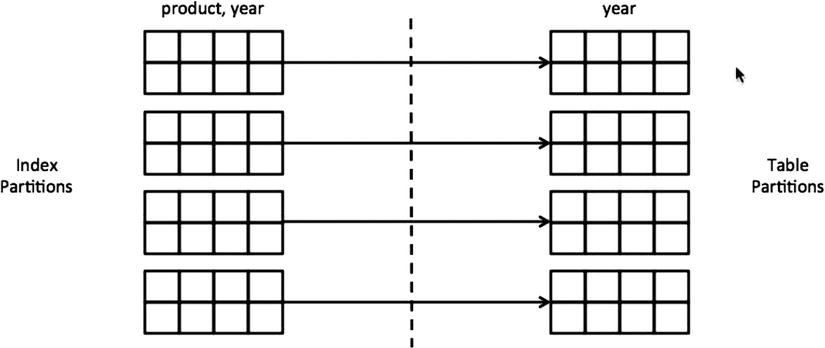
Figure 12-2. Local partitioned index
If the local index includes the partitioning key columns and if the SQL statement specifies predicates on the partitioning key columns, the execution plan needs to access just one or a few index partitions. This concept is known as partition elimination. Performance improves if the execution plan searches in a minimal number of partitions. In Listing 12-6, a partitioned table sales_fact_part is created with a partitioning key on the year column. A local index sales_fact_part_n1 is created on the product and year columns. First, the SELECT statement specifies the predicates on just the product column without specifying any predicate on the partitioning key column. In this case, all five index partitions must be accessed using the predicate product = 'Xtend Memory'. Columns Pstart and Pstop in the execution plan indicate that all partitions are accessed to execute this SQL statement.
Next, the SELECT statement in Listing 12-7 specifies the predicates on columns product and year. Using the predicate year=1998, the optimizer determines that only the second partition is to be accessed, eliminating access to all other partitions, because only the second partition stores the year column 1998 as indicated by the Pstart and Pstop columns in the execution plan. Also, the keywords in the execution plan TABLE ACCESS BY LOCAL INDEX ROWID BATCHED indicate that the row is accessed using a local index.
Listing 12-7. Local Indexes
drop table sales_fact_part;
CREATE table sales_fact_part
partition by range ( year )
( partition p_1997 values less than ( 1998) ,
  partition p_1998 values less than ( 1999),
  partition p_1999 values less than (2000),
  partition p_2000 values less than (2001),
  partition p_max values less than (maxvalue)
)
AS SELECT * from sales_fact;

create index sales_fact_part_n1 on sales_fact_part( product, year) local;

select * from  (
 select * from sales_fact_part where product = 'Xtend Memory'
) where rownum <21 ;

-----------------------------------------------------------------------
| Id  | Operation                | Name               | Pstart| Pstop |
-----------------------------------------------------------------------
|   0 | SELECT STATEMENT         |                    |       |       |
|*  1 |  COUNT STOPKEY           |                    |       |       |
|   2 |   PARTITION LIST ALL     |                    |     1 |     5 |
|   3 |    TABLE ACCESS BY LOCAL | SALES_FACT_PART    |     1 |     5 |
|     |     INDEX ROWID BATCHED  |                    |       |       |
|*  4 |     INDEX RANGE SCAN     | SALES_FACT_PART_N1 |     1 |     5 |
-----------------------------------------------------------------------

select * from  (
 select * from sales_fact_part where product = 'Xtend Memory' and year=1998
) where rownum <21 ;

-----------------------------------------------------------------------
| Id  | Operation                | Name               | Pstart| Pstop |
-----------------------------------------------------------------------
|   0 | SELECT STATEMENT         |                    |       |       |
|*  1 |  COUNT STOPKEY           |                    |       |       |
|   2 |   PARTITION LIST SINGLE  |                    |   KEY |   KEY |
|   3 |    TABLE ACCESS BY LOCAL | SALES_FACT_PART    |     1 |     1 |
|     |     INDEX ROWID BATCHED  |                    |       |       |
|*  4 |     INDEX RANGE SCAN     | SALES_FACT_PART_N1 |     1 |     1 |
-----------------------------------------------------------------------
Although the application availability is important, consider another point: If the predicate does not specify the partitioning key column, then all index partitions must be accessed to identify the candidate rows in the case of local indexes. This could lead to a performance issue if the partition count is very high, in the order of thousands. Even then, you want to measure the impact of creating the index as a local instead of a global index.
Creating local indexes improves the concurrency, too. I discuss this concept while discussing hash partitioning schemes.
Global Indexes
Global indexes are created with the keyword GLOBAL. In global indexes, partition boundaries of the index and the table do not need to match, and the partition keys can be different between the table and the index. Figure 12-3 shows how a global index bound does not have to match a table partition.
Figure 12-3. Global partitioned index
In Listing 12-8, a global index sales_fact_part_n1 is created on the year column. The partition boundaries are different between the table and the index, even though the partitioning column is the same. The subsequent SELECT statement specifies the predicate year=1998 to access the table, and the execution plan shows that partition 1 of the index and partition 2 of the table are accessed. Partition pruning was performed both at the table and index levels.
Listing 12-8. Global Indexes
create index sales_fact_part_n1 on sales_fact_part (year)
global partition by range ( year)
  (partition p_1998 values less than (1999),
   partition p_2000 values less than (2001),
   partition p_max values less than  (maxvalue)
);

select * from  (
 select * from sales_fact_part where product = 'Xtend Memory' and year=1998
) where rownum <21 ;

-----------------------------------------------------------------------
| Id  | Operation                | Name               | Pstart| Pstop |
-----------------------------------------------------------------------
|   0 | SELECT STATEMENT         |                    |       |       |
|*  1 |  COUNT STOPKEY           |                    |       |       |
|   2 |   PARTITION LIST SINGLE  |                    |     1 |     1 |
|   3 |    TABLE ACCESS BY LOCAL | SALES_FACT_PART    |     1 |     1 |
|     |     INDEX ROWID BATCHED  |                    |       |       |
|*  4 |     INDEX RANGE SCAN     | SALES_FACT_PART_N1 |     1 |     1 |
-----------------------------------------------------------------------
Maintenance on the global index leads to acquiring a higher level lock on the table, thereby reducing application availability. In contrast, maintenance can be done at the partition level in the local indexes, affecting only the corresponding table partition. In the example in Listing 12-8, rebuilding the index Sales_fact_part_n1 acquires a table-level lock in exclusive mode, leading to application downtime.
Unique indexes can be created as global indexes without including partitioning columns. But, the partitioning key of the table should be included in the case of local indexes to create a unique local index.
The partitioning scheme discussed so far is known as a range partitioning scheme. In this scheme, each partition stores rows with a range of partitioning column values. For example, clause partition p_2000 values less than (2001) specifies the upper boundary of the partition, so partition p_2000 stores rows with year column values less than 2001. The lower boundary of this partition is determined by the prior partition specification partition p_1998 values less than (1999). So, partition p_2000 stores the year column value range between 1999 and 2000.
Hash Partitioning vs. Range Partitioning
In the hash partitioning scheme, the partitioning key column values are hashed using a hashing algorithm to identify the partition to store the row. This type of partitioning scheme is appropriate for partitioning columns populated with artificial keys, such as rows populated with sequence-generated values. If the distribution of the column value is uniform, then all partitions store a nearly equal number of rows.
There are a few added advantages with the hash partitioning scheme. There is an administration overhead with the range partitioning scheme because new partitions need to be added regularly to accommodate future rows. For example, if the partitioning key is order date_column, then the new partitions must be added (or the partition with maxvalue specified must be split) to accommodate rows with future date values. With the hash partitioning scheme, the overhead is avoided because the rows are distributed equally among the partitions using a hashing algorithm. All partitions have nearly equal numbers of rows if the distribution of the column value is uniform and there is no reason to add more partitions regularly.
![]() Note Because of the nature of hashing algorithms, it is better to use a partition count of binary powers (in other words, 2, 4, 8, and so on). If you are splitting the partitions, it’s better to double the number of partitions to keep near equal-size partitions. If you do not do this, the partitions all have different numbers of rows, which defeats the purpose of partitioning.
Note Because of the nature of hashing algorithms, it is better to use a partition count of binary powers (in other words, 2, 4, 8, and so on). If you are splitting the partitions, it’s better to double the number of partitions to keep near equal-size partitions. If you do not do this, the partitions all have different numbers of rows, which defeats the purpose of partitioning.
Hash partitioned tables and indexes are effective in combating concurrency-related performance associated with unique and primary key indexes. It is typical of primary key columns to be populated using a sequence of generated values. Because the indexes store the column values in a sorted order, the column values for new rows go into the rightmost leaf block of the index. After that leaf block is full, subsequently inserted rows go into the new rightmost leaf block, with the contention point moving from one leaf block to another leaf block. As the concurrency of the insert into the table increases, sessions modify the rightmost leaf block of the index aggressively. Essentially, the current rightmost leaf block of that index is a major contention point. Sessions wait for block contention wait events such as buffer busy waits. In Real Application Clusters(RAC), this problem is magnified as a result of global cache communication overhead, and the event gc buffer busy becomes the top wait event. This type of index that grows rapidly on the right-hand side is called a right-hand growth index.
Concurrency issues associated with right-hand growth indexes can be eliminated by hash partitioning the index with many partitions. For example, if the index is partitioned by a hash with 32 partitions, then inserts are spread effectively among the 32 rightmost leaf blocks because there are 32 index trees (an index tree for an index partition). Partitioning the table using a hash partitioning scheme and then creating a local index on that partitioned table also has the same effect.
In Listing 12-9, a hash partitioned table sales_fact_part is created and the primary key id column is populated from the sequence sfseq. There are 32 partitions in this table with 32 matching index partitions for the sales_fact_part_n1 index, because the index is defined as a local index. The subsequent SELECT statement accesses the table with the predicate id=1000. The Pstart and Pstop columns in the execution plan show that partition pruning has taken place and only partition 25 is being accessed. The optimizer identifies partition 25 by applying a hash function on the column value 1000.
Listing 12-9. Hash Partitioning Scheme
drop sequence sfseq;
create sequence sfseq cache 200;

drop table sales_fact_part;
CREATE table sales_fact_part
partition by hash ( id )
partitions 32
AS SELECT sfseq.nextval id , f.* from sales_fact f;

create unique index sales_fact_part_n1 on sales_fact_part( id ) local;

select * from sales_fact_part where id =1000;
----------------------------------------------------------------------
| Id  | Operation               | Name               | Pstart| Pstop |
----------------------------------------------------------------------
|   0 | SELECT STATEMENT        |                    |       |       |
|   1 |  PARTITION HASH SINGLE  |                    |    25 |    25 |
|   2 |   TABLE ACCESS BY LOCAL | SALES_FACT_PART    |    25 |    25 |
|     |         INDEX ROWID     |                    |       |       |
|*  3 |    INDEX UNIQUE SCAN    | SALES_FACT_PART_N1 |    25 |    25 |
----------------------------------------------------------------------
If the data distribution is uniform in the partitioning key, as in the case of values generated from a sequence, then the rows are distributed uniformly to all partitions. You can use the dbms_rowid package to measure the data distribution in a hash partitioned table. In Listing 12-10, I use the dbms_rowid.rowid_objectcall to derive the object_id of the partition. Because every partition has its own object_id, you can aggregate the rows by object_id to measure the distribution of rows among the partitions. The output shows that all partitions have a nearly equal number of rows.
Listing 12-10. Hash Partitioning Distribution
select dbms_rowid.rowid_object(rowid) obj_id, count(*) from sales_fact_part
group by dbms_rowid.rowid_object(rowid);

OBJ_ID   COUNT(*)
------- ----------
  94855       3480
  94866       3320
  94873       3544
...
  94869       3495
  94876       3402
  94881       3555

32 rows selected.
Rows are distributed uniformly among partitions using the hashing algorithm. In a few cases, you might need to precalculate the partition where a row is to be stored. This knowledge is useful to improve massive loading of data into a hash partitioned table. As of Oracle Database version 12c, the ora_hash function can be used to derive the partition ID if supplied with a partition key value. For example, for a table with 32 partitions, ora_hash( column_name, 31, 0 ) returns the partition ID. The second argument to the ora_hash function is the partition count less one. In Listing 12-11, I use both ora_hash and dbms_rowid.rowid_object to show the mapping between object_id and the hashing algorithm output. A word of caution, though: In future releases of Oracle Database, you need to test this before relying on this strategy because the internal implementation of hash partitioned tables may change.
Listing 12-11. Hash Partitioning Algorithm
select dbms_rowid.rowid_object(rowid) obj_id, ora_hash ( id, 31, 0) part_id ,count(*)
from sales_fact_part
group by dbms_rowid.rowid_object(rowid), ora_hash(id,31,0)
order by 1;

OBJ_ID  PART_ID  COUNT(*)
------- -------- ---------
  94851        0      3505
  94852        1      3492
  94853        2      3572
...
  94880       29      3470
  94881       30      3555
  94882       31      3527

32 rows selected.
In essence, concurrency can be increased by partitioning the table and creating the right-hand growth indexes as local indexes. If the table cannot be partitioned, then that index alone can be partitioned to hash partitioning schema to resolve the performance issue.
Solutions to Match Application Characteristics
Oracle Database also provides indexing facilities to match the application characteristics. For example, some applications might be using function calls heavily, and SQL statements from those applications can be tuned using function-based indexes. I now discuss a few special indexing options available in Oracle Database.
Compressed indexes are a variation of the conventional B-tree indexes. This type of index is more suitable for columns with repeating values in the leading columns. Compression is achieved by storing the repeating values in the leading columns once in the index leaf block. Pointers from the row area point to these prefix rows, avoiding explicit storage of these repeating values in the row area. Compressed indexes can be smaller compared with conventional indexes if the column has many repeating values. There is a minor increase in CPU usage during the processing of compressed indexes, which can be ignored safely.
The simplified syntax for the compressed index specification clause is as follows:
Create index <index name> on <schema.table_name>
 ( col1 [,col2... coln] )
Compress N Storage-parameter-clause
;
The number of leading columns to compress can be specified while creating a compressed index using the syntax compress N. For example, to compress two leading columns in a three-column index, the clause compress 2 can be specified. Repeating values in the first two columns are stored in the prefix area just once. You can only compress the leading columns; for example, you can’t compress columns 1 and 3.
In Listing 12-12, a compressed index sales_fact_c1 is created on columns product, year, and week, with a compression clause compress 2 specified to compress the two leading columns. In this example, the repeating values of the product and year columns are stored once in the leaf blocks because the compress 2 clause is specified. Because there is higher amount of repetition in these two column values, the index size is reduced from 6MB (conventional index) to 2MB (compressed index) by compressing these two leading columns.
Listing 12-12. Compressed Indexes
  select * from  (
    select product, year,week, sale from sales_fact
    order by product, year,week
  ) where rownum <21;

PRODUCT                              YEAR  WEEK       SALE
------------------------------ ---------- ----- ----------
1.44MB External 3.5" Diskette        1998     1       9.71
1.44MB External 3.5" Diskette        1998     1      38.84
1.44MB External 3.5" Diskette        1998     1       9.71
...

create index sales_fact_c1 on sales_fact ( product, year, week);

select 'Compressed index size (MB) :' ||trunc(bytes/1024/1024, 2)
from user_segments where segment_name='SALES_FACT_C1';

Compressed index size (MB) :6
...
create index sales_fact_c1 on sales_fact ( product, year, week) compress 2;

select 'Compressed index size (MB) :' ||trunc(bytes/1024/1024,2)
from user_segments where segment_name='SALES_FACT_C1';

Compressed index size (MB) :2
In Figure 12-4, a high-level overview of a compressed index leaf block is shown. This compressed index is a two-column index on the continent and country columns. Repeating values of continent columns are stored once in the prefix area of the index leaf blocks because the index is created with the clause compress 1. Pointers are used from the row area pointing to the prefix rows. For example, the continent column value ASIA occurs in three rows—(Asia, Hong Kong), (Asia, India), and (Asia, Indonesia)—but is stored once in the prefix area, and these three rows reuse the continent column value, avoiding explicit storage of the value three times. This reuse of column values reduces the size of the index.
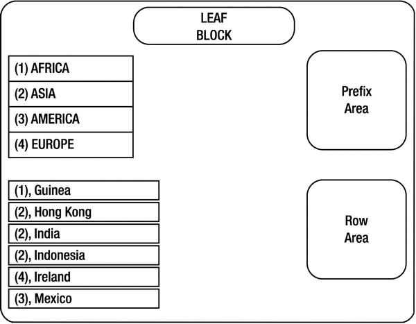
Figure 12-4. Compressed index
It is evident that data properties play a critical role in the compression ratio. If the repetition count of the column values is higher, then the compressed indexes provide greater benefit. If there is no repetition, then the compressed index might be bigger than the conventional index. So, compressed indexes are suitable for indexes with fewer distinct values in the leading columns. Columns compression and prefix_length in the dba_indexes/user_indexes view shows the compression attributes of the indexes.
The number of columns to choose for compression depends on the column value distribution. To identify the optimal number of columns to compress, the analyze index/validate structure statement can be used. In Listing 12-13, an uncompressed index sales_fact_c1 is analyzed with the validate structure clause. This analyze statement populates the index_stats view. The column index_stats.opt_cmpr_count displays the optimal compression count; for this index, it’s 2. The column index_stats.cmpr_pctsave displays the index size savings compressing with the opt_cmpr_count columns. In this example, there is a savings of 67 percent in index space usage; so, the size of the compressed index with the compress 2 clause is 33 percent of the conventional uncompressed index size. This size estimate computes to 1.98MB and is close enough to actual index size.
Listing 12-13. Optimal Compression Count
analyze index sales_fact_c1 validate structure;

select opt_cmpr_count, opt_cmpr_pctsave from index_stats
where name ='SALES_FACT_C1';

OPT_CMPR_COUNT OPT_CMPR_PCTSAVE
-------------- ----------------
-------------2 --------------67
Beware that the analyze index validate structure statement acquires a share-level lock on the table and might induce application downtime.
There are a few restrictions on compressed indexes. For example, all columns can be compressed in the case of nonunique indexes, and all but the last column can be compressed in the case of unique indexes.
Function-Based Indexes
If a predicate applies a function on an indexed column, then the index on that column might not be chosen by the optimizer. For example, the index on the id column may not be chosen for the predicate to_char(id)= ‘1000’ because the to_char function is applied on the indexed column. This restriction can be overcome by creating a function-based index on the expression to_char(id). Function-based indexes prestore the results of functions. Expressions specified in the predicate must match the expressions specified in the function-based index, though.
A function-based index can be created on user-defined functions, but those functions must be defined as deterministic functions—meaning, they must always return a consistent value for every execution of the function. User-defined functions that do not adhere to this rule can’t be used to create the function-based indexes.
In Listing 12-14, a SELECT statement accesses the sales_fact_part table using the clause to_char(id)= ‘1000’. Without a function-based index, the optimizer chooses a full table scan access plan. A function-based index fact_part_fbi1 with the expression to_char(id) is added, and the optimizer chooses an index-based access path for the SELECT statement.
Listing 12-14. Function-Based Index
drop index sales_fact_part_fbi1;
select * from sales_fact_part where to_char(id)='1000';

--------------------------------------------------------------
| Id  | Operation          | Name            | Pstart| Pstop |
--------------------------------------------------------------
|   0 | SELECT STATEMENT   |                 |       |       |
|   1 |  PARTITION HASH ALL|                 |     1 |    32 |
|*  2 |   TABLE ACCESS FULL| SALES_FACT_PART |     1 |    32 |
--------------------------------------------------------------

create index sales_fact_part_fbi1 on sales_fact_part( to_char(id)) ;
@analyze_table_sfp
select * from sales_fact_part where to_char(id)='1000';

------------------------------------------------------------------------
| Id  | Operation               | Name                 | Pstart| Pstop |
------------------------------------------------------------------------
|   0 | SELECT STATEMENT        |                      |       |       |
|   1 |  TABLE ACCESS BY GLOBAL | SALES_FACT_PART      | ROWID | ROWID |
|     |    INDEX ROWID BATCHED  |                      | ROWID | ROWID |
|*  2 |   INDEX RANGE SCAN      | SALES_FACT_PART_FBI1 |       |       |
------------------------------------------------------------------------

Predicate Information (identified by operation id):
---------------------------------------------------

   2 - access("SALES_FACT_PART"."SYS_NC00009$"='1000')
Note the access predicates printed at the end of Listing 12-14: "SYS_NC00009$"='1000'. A few implementation details of the function-based indexes are presented in Listing 12-15. Function-based indexes add a virtual column, with the specified expression as the default value, and then index that virtual column. This virtual column is visible in the dba_tab_cols view, and the dba_tab_cols.data_default column shows that expression used to populate the virtual column. Further viewing of dba_ind_columns shows that the virtual column is indexed.
Listing 12-15. Virtual Columns and Function-Based Index
select data_default, hidden_column, virtual_column from dba_tab_cols
where table_name='SALES_FACT_PART' and virtual_column='YES';

DATA_DEFAULT                   HID VIR
------------------------------ --- ---
TO_CHAR("ID")                  YES YES

select index_name,column_name from dba_ind_columns
where index_name='SALES_FACT_PART_FBI1';

INDEX_NAME                     COLUMN_NAME
------------------------------ -------------
SALES_FACT_PART_FBI1           SYS_NC00009$
It is important to collect statistics on the table after adding a function-based index. If not, that new virtual column does not have statistics, which might lead to performance anomalies. The script analyze_table_sfp.sql is used to collect statistics on the table with cascade=>true. Listing 12-16 shows the contents of the script analyze_table_sfp.sql.
Listing 12-16. analyze_table_sfp.sql
begin
   dbms_stats.gather_table_stats (
   ownname =>user,
   tabname=>'SALES_FACT_PART',
   cascade=>true);
end;
/
Function-based indexes can be implemented using virtual columns explicitly, too. An index can be added over that virtual column optionally. The added advantage with this method is that you can also use a partitioning scheme with a virtual column as the partitioning key. In Listing 12-17, a new virtual column, id_char, is added to the table using the VIRTUAL keyword. Then, a globally partitioned index on the id_char virtual column is created. The execution plan of the SELECT statement shows that table is accessed using the new index, and the predicate to_char(id)='1000' is rewritten to use the virtual column with the predicate id_char='1000'.
Listing 12-17. Virtual Columns and Function-Based Index
alter table sales_fact_part add
 ( id_char varchar2(40) generated always as (to_char(id) ) virtual );

create index sales_fact_part_c1 on sales_fact_part ( id_char)
global partition by hash (id_char)
partitions 32 ;

@analyze_table_sfp
select * from sales_fact_part where to_char(id)='1000' ;

--------------------------------------------------------------------------
| Id  | Operation                                   | Name               |
--------------------------------------------------------------------------
|   0 | SELECT STATEMENT                            |                    |
|   1 |  PARTITION HASH SINGLE                      |                    |
|   2 |   TABLE ACCESS BY GLOBAL INDEX ROWID BATCHED| SALES_FACT_PART    |
|*  3 |    INDEX RANGE SCAN                         | SALES_FACT_PART_C1 |
--------------------------------------------------------------------------

Predicate Information (identified by operation id):
---------------------------------------------------

   3 - access("SALES_FACT_PART"."ID_CHAR"='1000')
Reverse Key Indexes
Reverse key indexes were introduced by Oracle as another option to combat performance issues associated with right-hand growth indexes discussed in “Hash Partitioning vs. Range Partitioning.” In reverse key indexes, column values are stored in reverse order, character by character. For example, column value 12345 is stored as 54321 in the index. Because the column values are stored in reverse order, consecutive column values are stored in different leaf blocks of the index, thereby avoiding the contention issues with right-hand growth indexes. In the table blocks, these column values are stored as 12345, though.
There are two issues with reverse key indexes:
- The range scan on reverse key indexes is not possible for range operators such as between, less than, greater than, and so on. This is understandable because the underlying assumption of an index range scan is that column values are stored in ascending or descending logical key order. Reverse key indexes break this assumption because the column values are stored in the reverse order, no logical key order is maintained, and so index range scans are not possible with reverse key indexes.
- Reverse key indexes can increase physical reads artificially because the column values are stored in numerous leaf blocks and those leaf blocks might need to be read into the buffer cache to modify the block. But, the cost of this increase in IO should be measured against the concurrency issues associated with right-hand growth indexes.
In Listing 12-18, a reverse key index Sales_fact_part_n1 is created with a REVERSE keyword. First, the SELECT statement with the predicate id=1000 uses the reverse key index, because equality predicates can use reverse key indexes. But, the next SELECT statement with the predicate id between 1000 and 1001 uses the full table scan access path because the index range scan access path is not possible with reverse key indexes.
Listing 12-18. Reverse Key Indexes
drop index sales_fact_part_n1;
create unique index sales_fact_part_n1 on sales_fact_part ( id ) global  reverse ;

select * from sales_fact_part where id=1000;

---------------------------------------------------------------------
| Id  | Operation              | Name               | Pstart| Pstop |
---------------------------------------------------------------------
|   0 | SELECT STATEMENT       |                    |       |       |
|   1 |  TABLE ACCESS BY GLOBAL| SALES_FACT_PART    |    25 |    25 |
|     |     INDEX ROWID        |                    |       |       |
|*  2 |   INDEX UNIQUE SCAN    | SALES_FACT_PART_N1 |       |       |
---------------------------------------------------------------------

select * from sales_fact_part where id between 1000 and 1001;

--------------------------------------------------------------
| Id  | Operation          | Name            | Pstart| Pstop |
--------------------------------------------------------------
|   0 | SELECT STATEMENT   |                 |       |       |
|   1 |  PARTITION HASH ALL|                 |     1 |    32 |
|*  2 |   TABLE ACCESS FULL| SALES_FACT_PART |     1 |    32 |
--------------------------------------------------------------
Especially in RAC, right-hand growth indexes can cause intolerable performance issues. Reverse key indexes were introduced to combat this performance problem, but you should probably consider hash partitioned indexes instead of reverse key indexes.
Descending Indexes
Indexes store column values in ascending order by default; this can be switched to descending order using descending indexes. If your application fetches the data in a specific order, then the rows need to be sorted before the rows are sent to the application. These sorts can be avoided using descending indexes. These indexes are useful if the application is fetching the data millions of times in a specific order—for example, customer data fetched from the customer transaction table in the reverse chronological order.
In Listing 12-19, an index Sales_fact_c1 together with the columns product desc, year desc, week desc specifies a descending order for these three columns. The SELECT statement accesses the table by specifying an ORDER BY clause with the sort order product desc, year desc, week desc matching the index sort order. The execution plan shows there is no sort step, even though there is an ORDER BY clause in the SELECT statement.
Listing 12-19. Descending Indexes
drop index sales_fact_c1;
create index sales_fact_c1 on sales_fact
( product desc, year desc, week desc ) ;

@analyze_sf.sql

select year, week from sales_fact s
where year in ( 1998,1999,2000) and week<5 and product='Xtend Memory'
order by product desc,year desc, week desc ;

-----------------------------------------------------------------
| Id  | Operation         | Name          | E-Rows | Cost (%CPU)|
-----------------------------------------------------------------
|   0 | SELECT STATEMENT  |               |        |     5 (100)|
|   1 |  INLIST ITERATOR  |               |        |            |
|*  2 |   INDEX RANGE SCAN| SALES_FACT_C1 |    109 |     5   (0)|
-----------------------------------------------------------------

select index_name, index_type from dba_indexes
where index_name='SALES_FACT_C1';

INDEX_NAME                     INDEX_TYPE
------------------------------ ------------------------------
SALES_FACT_C1                  FUNCTION-BASED NORMAL
Descending indexes are implemented as a function-based index as of Oracle Database release 11gR2.
Solutions to Management Problems
Indexes can be used to resolve operational problems faced in the real world. For example, to see the effects of a new index on a production application, you can use invisible indexes. You can also use invisible indexes to drop the indexes safely or, if working with Exadata, to test whether the indexes are still needed.
Invisible Indexes
In certain scenarios, you might want to add an index to tune the performance of a SQL statement, but you may not be sure about the negative impact of the index. Invisible indexes are useful to measure the impact of a new index with less risk. An index can be added to the database marked as invisible, and the optimizer does not choose that index. You can make an index invisible to ensure there is no negative consequence of the absence of the index.
After adding the index to the database, you can set a parameter optimizer_use_invisible_indexes to TRUE in your session without affecting the application performance, and then review the execution plan of the SQL statement. In Listing 12-20, the first SELECT statement uses the index sales_fact_c1 in the execution plan. The next SQL statement marks the sales_fact_c1 index as invisible, and the second execution plan of the same SELECT statement shows that the index is ignored by the optimizer.
Listing 12-20. Invisible Indexes
select * from  (
 select * from sales_fact where product = 'Xtend Memory' and year=1998 and week=1
) where rownum <21 ;

-----------------------------------------------------------------------------
| Id  | Operation                            | Name          | Rows  | Bytes|
-----------------------------------------------------------------------------
|   0 | SELECT STATEMENT                     |               |     7 |   490|
|*  1 |  COUNT STOPKEY                       |               |       |      |
|   2 |   TABLE ACCESS BY INDEX ROWID BATCHED| SALES_FACT    |     7 |   490|
|*  3 |    INDEX RANGE SCAN                  | SALES_FACT_C1 |     9 |      |
-----------------------------------------------------------------------------

alter index sales_fact_c1 invisible;

select * from  (
 select * from sales_fact where product = 'Xtend Memory' and year=1998 and week=1
) where rownum <21;

---------------------------------------------------------
| Id  | Operation          | Name       | Rows  | Bytes |
---------------------------------------------------------
|   0 | SELECT STATEMENT   |            |     7 |   490 |
|*  1 |  COUNT STOPKEY     |            |       |       |
|*  2 |   TABLE ACCESS FULL| SALES_FACT |     7 |   490 |
---------------------------------------------------------
In Listing 12-20, the execution plan shows that the optimizer chooses the sales_fact_c1 index after setting the parameter to TRUE at the session level.
There is another use case for invisible indexes. These indexes are useful to reduce the risk while dropping unused indexes. It is not a pleasant experience to drop unused indexes from a production database, only to realize later that the dropped index is used in an important report. Even after performing extensive analysis, it is possible that the dropped index might be needed for a business process, and recreating indexes might lead to application downtime. From Oracle Database version 11g onward, you can mark the index as invisible, wait for few weeks, and then drop the index with less risk if no process is affected. If the index is needed after marking it as invisible, then that index can be reverted quickly to visible with just a SQL statement.
Listing 12-21. optimizer_use_invisible_indexes
alter session set optimizer_use_invisible_indexes = true;
select * from  (
 select * from sales_fact where product = 'Xtend Memory' and year=1998 and week=1
) where rownum <21 ;

-----------------------------------------------------------------------------
| Id  | Operation                            | Name          | Rows  | Bytes|
-----------------------------------------------------------------------------
|   0 | SELECT STATEMENT                     |               |     7 |   490|
|*  1 |  COUNT STOPKEY                       |               |       |      |
|   2 |   TABLE ACCESS BY INDEX ROWID BATCHED| SALES_FACT    |     7 |   490|
|*  3 |    INDEX RANGE SCAN                  | SALES_FACT_C1 |     9 |      |
-----------------------------------------------------------------------------
Invisible indexes are maintained during DML activity similar to any other indexes. This operational feature is useful in reducing the risk associated with dropping indexes.
Virtual Indexes
Have you ever added an index only to realize later that the index is not chosen by the optimizer because of data distribution or some statistics issue? Virtual indexes are useful to review the effectiveness of an index. Virtual indexes do not have storage allocated and, so, can be created quickly. Virtual indexes are different from invisible indexes in that invisible indexes have storage associated with them, but the optimizer cannot choose them; virtual indexes do not have storage segments associated with them. For this reason, virtual indexes are also called nosegment indexes.
The session-modifiable underscore parameter _use_nosegment_indexes controls whether the optimizer can consider a virtual index. This parameter is FALSE by default, and the application does not choose virtual indexes. You can test the virtual index using the following method without affecting other application functionality: create the index, enable the parameter to TRUE in your session, and verify the execution plan of the SQL statement. In Listing 12-22, a virtual index sales_virt was created with the nosegment clause. After modifying the parameter to TRUE in the current session, the execution plan of the SELECT statement is checked. The execution plan shows that this index is chosen by the optimizer for this SQL statement. After reviewing the plan, this index can be dropped and recreated as a conventional index.
Listing 12-22. Virtual Indexes
create index sales_virt on sales ( cust_id, promo_id) nosegment;

alter session set "_use_nosegment_indexes"=true;

explain plan for
select * from sh.sales
where cust_id=:b1 and promo_id=:b2;

select * from table(dbms_xplan.display) ;

-----------------------------------------------------------------------------
| Id  | Operation                                  | Name       | Cost(%CPU)|
-----------------------------------------------------------------------------
|   0 | SELECT STATEMENT                           |            |     9  (0)|
|   1 |  TABLE ACCESS BY GLOBAL INDEX ROWID BATCHED| SALES      |     9  (0)|
|*  2 |   INDEX RANGE SCAN                         | SALES_VIRT |     1  (0)|
-----------------------------------------------------------------------------
Virtual indexes do not have storage associated with them, so these indexes are not maintained. But, you can collect statistics on these indexes as if they are conventional indexes. Virtual indexes can be used to improve the cardinality estimates of predicates without incurring the storage overhead associated with conventional indexes.
Bitmap Join Indexes
Bitmap join indexes are useful in data warehouse applications to materialize the joins between fact and dimension tables. In data warehouse tables, fact tables are typically much larger than the dimension tables, and the dimension and fact tables are joined using a primary key, with a foreign key relationship between them. These joins are costlier because of the size of the fact tables, and performance can be improved for these queries if the join results can be prestored. Materialized views are one option to precalculate the join results; bitmap join indexes are another option.
In Listing 12-23, a typical data warehouse query and its execution plan is shown. The sales table is a fact table and the other tables are dimension tables in this query. The sales table is joined to other dimension tables by primary key columns on the dimension tables. The execution plan shows the sales table is the leading table in this join processing, and the other dimension tables are joined to derive the final result set. These are the four join operations in this execution plan. This execution plan can be very costly if the fact table is huge.
Listing 12-23. A Typical Data Warehouse Query
select sum(s.quantity_sold), sum(s.amount_sold)
  from sales s, products p, customers c, channels ch
where s.prod_id = p.prod_id and
     s.cust_id = c.cust_id and
     s.channel_id = ch.channel_id and
     p.prod_name='Y box' and
     c.cust_first_name='Abigail' and
     ch.channel_desc = 'Direct_sales' ;

-----------------------------------------------------------------------------
| Id | Operation                            | Name             |Rows  |Bytes|
-----------------------------------------------------------------------------
|  0 | SELECT STATEMENT                     |                  |    1 |   75|
|  1 |  SORT AGGREGATE                      |                  |    1 |   75|
|* 2 |   HASH JOIN                          |                  |   10 |  750|
|* 3 |    TABLE ACCESS FULL                 | CUSTOMERS        |   43 |  516|
|  4 |    NESTED LOOPS                      |                  |      |     |
|  5 |     NESTED LOOPS                     |                  | 1595 |   8K|
|  6 |      MERGE JOIN CARTESIAN            |                  |    1 |   43|
|* 7 |       TABLE ACCESS FULL              | PRODUCTS         |    1 |   30|
|  8 |       BUFFER SORT                    |                  |    1 |   13|
|* 9 |        TABLE ACCESS FULL             | CHANNELS         |    1 |   13|
| 10 |      PARTITION RANGE ALL             |                  |      |     |
| 11 |       BITMAP CONVERSION TO ROWIDS    |                  |      |     |
| 12 |        BITMAP AND                    |                  |      |     |
|*13 |         BITMAP INDEX SINGLE VALUE    | SALES_PROD_BIX   |      |     |
|*14 |         BITMAP INDEX SINGLE VALUE    | SALES_CHANNEL_BIX|      |     |
| 15 |     TABLE ACCESS BY LOCAL INDEX ROWID| SALES            | 3190 |63800|
-----------------------------------------------------------------------------
In Listing 12-24, a bitmap join index Sales_bji1 is created to precalculate the join results. Notice the index creation statement joins the sales and dimension tables similar to the join predicates specified in the query. The SELECT statement is reexecuted after creating the index, and the execution plan of the SELECT statement shows access to the bitmap join index, followed by access to the sales table without any join processing. Internally, three new virtual columns are added to this table, and an index is created on these three virtual columns. In a nutshell, the bitmap join index materializes the result set with the indexes on the virtual columns, thereby avoiding costly join processing.
Listing 12-24. Bitmap Join Index
alter table products modify primary key validate;

alter table customers modify primary key validate;

alter table channels modify primary key validate;

create bitmap index sales_bji1 on sales ( p.prod_name, c.cust_first_name, ch.channel_desc)
from sales s, products p, customers c, channels ch
where s.prod_id = p.prod_id and
      s.cust_id = c.cust_id and
      s.channel_id = ch.channel_id
LOCAL ;

select sum(s.quantity_sold), sum(s.amount_sold)
  from sales s, products p, customers c, channels ch
where s.prod_id = p.prod_id and
     s.cust_id = c.cust_id and
     s.channel_id = ch.channel_id and
     p.prod_name='Y box' and
     c.cust_first_name='Abigail' and
     ch.channel_desc = 'Direct_sales';

--------------------------------------------------------------------------
| Id  | Operation                           | Name       | Rows  | Bytes |
--------------------------------------------------------------------------
|   0 | SELECT STATEMENT                    |            |     1 |    20 |
|   1 |  SORT AGGREGATE                     |            |     1 |    20 |
|   2 |   PARTITION RANGE ALL               |            |    19 |   380 |
|   3 |    TABLE ACCESS BY LOCAL INDEX      | SALES      |    19 |   380 |
|     |        ROWID BATCHED                |            |       |       |
|   4 |     BITMAP CONVERSION TO ROWIDS     |            |       |       |
|*  5 |      BITMAP INDEX SINGLE VALUE      | SALES_BJI1 |       |       |
--------------------------------------------------------------------------
There are a few restrictions on bitmap join indexes: all dimensions need to have validated primary or unique constraints defined, the index must be local, and so on. The first three statements in Listing 12-24 modify the constraint state to validated to enable creation of a bitmap join index.
Bitmap join indexes are useful in data warehouse environments, adhering to a good data model. These indexes are not useful in OLTP applications, though.
Summary
A good choice of index type and an optimal choice of indexed columns are essential to maintaining application performance. Armed with this new knowledge of various index types, you should focus on matching index types to application access paths. Because Oracle Database provides rich index functionality, it is best to use optimal index types to suit your application access patterns. It’s also vitally important to add indexes only when necessary. Unnecessary indexes waste space, increase redo size and undo size, and waste valuable CPU cycles and memory.