Column 10: Squeezing Space

If you’re like several people I know, your first thought on reading the title of this column is, “How quaint!” In the bad old days of computing, so the story goes, programmers were constrained by small machines, but those days are long gone. The new philosophy is, “A gigabyte here, a gigabyte there, pretty soon you’re talking about real memory.” And there is truth in that view — many programmers use big machines and rarely have to worry about squeezing space from their programs.

But every now and then, thinking hard about compact programs can be profitable. Sometimes the thought gives new insight that makes the program simpler. Reducing space often has desirable side-effects on run time: smaller programs are faster to load and fit more easily into a cache, and less data to manipulate usually means less time to manipulate it. The time required to transmit data across a network is usually directly proportional to the size of the data. Even with cheap memories, space can be critical. Tiny machines (such as those found in toys and household appliances) still have tiny memories. When huge machines are used to solve huge problems, we must still be careful with memory.

Keeping perspective on its importance, let’s survey a few important techniques for reducing space.

Fred Brooks observed the power of simplification when he wrote a payroll program for a national company in the mid 1950’s. The bottleneck of the program was the representation of the Kentucky state income tax. The tax was specified in the law by a two-dimensional table with income as one dimension, and number of exemptions as the other. Storing the table explicitly required thousands of words of memory, more than the capacity of the machine.

The first approach Brooks tried was to fit a mathematical function through the tax table, but it was so jagged that no simple function would come close. Knowing that it was made by legislators with no predisposition to crazy mathematical functions, Brooks consulted the minutes of the Kentucky legislature to see what arguments had led to the bizarre table. He found that the Kentucky tax was a simple function of the income that remained after federal tax was deducted. His program therefore calculated federal tax from existing tables, and then used the remaining income and a table of just a few dozen words of memory to find the Kentucky tax.

By studying the context in which the problem arose, Brooks was able to replace the original problem to be solved with a simpler problem. While the original problem appeared to require thousands of words of data space, the modified problem was solved with a negligible amount of memory.

Simplicity can also reduce code space. Column 3 describes several large programs that were replaced by small programs with more appropriate data structures. In those cases, a simpler view of the program reduced the source code from thousands to hundreds of lines and probably also shrank the size of the object code by an order of magnitude.

In the corresponding map, point 17 is in location (0, 2), point 538 is in (0, 5), and the four other visible locations in the first column are empty.

The array was easy to implement and gave rapid access time. The programmer had the choice of implementing each integer in 16 or 32 bits. Had he chosen 32-bit integers, the 200×200 = 40,000 elements would have consumed 160 kilobytes. He therefore chose the shorter representation, and the array used 80 kilobytes, or one-sixth of the half-megabyte memory. Early in the life of the system that was no problem. As the system grew, though, it started to run out of space. The programmer asked me how we might reduce the storage devoted to this structure. How would you advise the programmer?

This is a classic opportunity for using a sparse data structure. This example is old, but I’ve seen the same story recently in representing a 10,000×10,000 matrix with a million active entries on a hundred-megabyte computer.

An obvious representation of sparse matrices uses an array to represent all columns, and linked lists to represent the active elements in a given column. This picture has been rotated 90 degrees clockwise for a prettier layout:

This picture shows three points in the first column: point 17 is in (0, 2), point 538 is in (0, 5), and point 1053 is in (0,126). Two points are in column 2, and none are in column 3. We search for the point (i, j) with this code:

Click here to view code image

for (p = colhead[i]; p != NULL; p = p->next)
    if p->row == j
        return p->pointnum
return -1

Looking up an array element visits at most 200 nodes in the worst case, but only about ten nodes on the average.

This structure uses an array of 200 pointers and also 2000 records, each with an integer and two pointers. The model of space costs in Appendix 3 tells us that the pointers will occupy 800 bytes. If we allocate the records as a 2000-element array, they will occupy 12 bytes each, for a total of 24,800 bytes. (If we were to use the default malloc described in that appendix, though, each record would consume 48 bytes, and the overall structure would in fact increase from the original 80 kilobytes to 96.8 kilobytes.)

The programmer had to implement the structure in a version of Fortran that did not support pointers and structures. We therefore used an array of 201 elements to represent the columns, and two parallel arrays of 2000 elements to represent the points. Here are those three arrays, with the integer indices in the bottom array also depicted as arrows. (The 1-indexed Fortran arrays have been changed to use 0-indexing for consistency with the other arrays in this book.)

The points in column i are represented in the row and pointnum arrays between locations firstincol[i] and firstincol[i + 1]–1; even though there are only 200 columns, firstincol[200] is defined to make this condition hold. To determine what point is stored in position (i, j) we use this pseudocode:

Click here to view code image

for k = [firstincol[i], firstincol[i+1])
    if row[k] == j
        return pointnum[k]
return -1

This version uses two 2000-element arrays and one 201-element array. The programmer implemented exactly this structure, using 16-bit integers for a total of 8402 bytes. It is a little slower than using the complete matrix (about ten node visits on the average). Even so, the program had no trouble keeping up with the user. Because of the good module structure of the system, this approach was incorporated in a few hours by changing a few functions. We observed no degradation in run time and gained 70 sorely needed kilobytes.

Had the structure still been a space hog, we could have reduced its space even further. Because the elements of the row array are all less than 200, they can each be stored in a single-byte unsigned char, this reduces the space to 6400 bytes. We could even remove the row array altogether, if the row is already stored with the point itself:

Click here to view code image

for k = [firstincol[i], firstincol[i+1])
    if point[pointnum[k]].row == j
        return pointnum[k]
return -1

This reduces the space to 4400 bytes.

In the real system, rapid lookup time was critical both for user interaction and because other functions looked up points through the same interface. If run time had not been important and if the points had row and col fields, then we could have achieved the ultimate space reduction to zero bytes by sequentially searching through the array of points. Even if the points did not have those fields, the space for the structure could be reduced to 4000 bytes by “key indexing”: we scan through an array in which the i^th element contains two one-byte fields that give the row and col values of point i.

This problem illustrates several general points about data structures. The problem is classic: sparse array representation (a sparse array is one in which most entries have the same value, usually zero). The solution is conceptually simple and easy to implement. We used a number of space-saving measures along the way. We need no lastincol array to go with firstincol; we instead use the fact that the last point in this column is immediately before the first point in the next column. This is a trivial example of recomputing rather than storing. Similarly, there is no col array to go with row, because we only access row through the firstincol array, we always know the current column. Although row started with 32 bits, we reduced its representation to 16 and finally 8 bits. We started with records, but eventually went to arrays to squeeze out a few kilobytes here and there.

Don’t Store, Recompute. The space required to store a given object can be dramatically reduced if we don’t store it but rather recompute it whenever it is needed. This is exactly the idea behind doing away with the matrix of points, and performing a sequential search each time from scratch. A table of the prime numbers might be replaced by a function for testing primality. This method trades more run time for less space, and it is applicable only if the objects to be “stored” can be recomputed from their description.

Such “generator programs” are often used in executing several programs on identical random inputs, for such purposes as performance comparisons or regression tests of correctness. Depending on the application, the random object might be a file of randomly generated lines of text or a graph with randomly generated edges. Rather than storing the entire object, we store just its generator program and the random seed that defines the particular object. By taking a little more time to access them, huge objects can be represented in a few bytes.

Users of PC software may face such a choice when they install software from a CD-ROM or DVD-ROM. A “typical” installation might store hundreds of megabytes of data on the system’s hard drive, where it can be read quickly. A “minimal” installation, on the other hand, will keep those files on the slower device, but will not use the disk space. Such an installation conserves magnetic disk space by using more time to read the data each time the program is invoked.

For many programs that run across networks, the most pressing concern about data size is the time it will take to transmit it. We can sometimes decrease the amount of data transmitted by caching it locally, following the dual advice of “Store, don’t retransmit.”

Sparse Data Structures. Section 10.2 introduced these structures. In Section 3.1 we saved space by storing a “ragged” three-dimensional table in a two-dimensional array. If we use a key to be stored as an index into a table, then we need not store the key itself; rather, we store only its relevant attributes, such as a count of how many times it has been seen. Applications of this key indexing technique are described in the catalog of algorithms in Appendix 1. In the sparse matrix example above, key indexing through the firstincol array allowed us to do without a col array.

Storing pointers to shared large objects (such as long text strings) removes the cost of storing many copies of the same object, although one has to be careful when modifying a shared object that all its owners desire the modification. This technique is used in my desk almanac to provide calendars for the years 1821 through 2080; rather than listing 260 distinct calendars it gives fourteen canonical calendars (seven days of the week for January 1 times leap year or non-leap year) and a table giving a calendar number for each of the 260 years.

Some telephone systems conserve communication bandwidth by viewing voice conversations as a sparse structure. When the volume in one direction falls below a critical level, silence is transmitted using a succinct representation, and the bandwidth thus saved is used to transmit other conversations.

Data Compression. Insights from information theory reduce space by encoding objects compactly. In the sparse matrix example, for instance, we compressed the representation of a row number from 32 to 16 to 8 bits. In the early days of personal computers, I built a program that spent much of its time reading and writing long strings of decimal digits. I changed it to encode the two decimal digits a and b in one byte (instead of the obvious two) by the integer c = 10×a+b. The information was decoded by the two statements

a = c / 10
b = c % 10

This simple scheme reduced the input/output time by half, and also squeezed a file of numeric data onto one floppy disk instead of two. Such encodings can reduce the space required by individual records, but the small records might take more time to encode and decode (see Problem 6).

Information theory can also compress a stream of records being transmitted over a channel such as a disk file or a network. Sound can be recorded at CD-quality by recording two channels (stereo) at 16-bit accuracy at 44,100 samples per second. One second of sound requires 176,400 bytes using this representation. The MP3 standard compresses typical sound files (especially music) to a small fraction of that size. Problem 10.10 asks you to measure the effectiveness of several common formats for representing text, images, sounds and the like. Some programmers build special-purpose compression algorithms for their software; Section 13.8 sketches how a file of 75,000 English words was squeezed into 52 kilobytes.

Allocation Policies. Sometimes how much space you use isn’t as important as how you use it. Suppose, for instance, that your program uses three different types of records, x, y and z, all of the same size. In some languages your first impulse might be to declare, say, 10,000 objects of each of the three types. But what if you used 10,001 x’s and no y’s or z’s? The program could run out of space after using 10,001 records, even though 20,000 others were completely unused. Dynamic allocation of records avoids such obvious waste by allocating records as they are needed.

Dynamic allocation says that we shouldn’t ask for something until we need it; the policy of variable-length records says that when we do ask for something, we should ask for only as much as we need. In the old punched-card days of eighty-column records it was common for more than half the bytes on a disk to be trailing blanks. Variable-length files denote the end of lines by a newline character and thereby double the storage capacity of such disks. I once tripled the speed of an input/output-bound program by using records of variable length: the maximum record length was 250, but only about 80 bytes were used on the average.

Garbage collection recycles discarded storage so that the old bits are as good as new. The Heapsort algorithm in Section 14.4 overlays two logical data structures used at separate times in the same physical storage locations.

In another approach to sharing storage, Brian Kernighan wrote a traveling salesman program in the early 1970’s in which the lion’s share of the space was devoted to two 150×150 matrices. The two matrices, which I’ll call a and b to protect their anonymity, represented distances between points. Kernighan therefore knew that they had zero diagonals (a[i,i] = 0) and that they were symmetric (a[i, j] = a[j, i]). He therefore let the two triangular matrices share space in one square matrix, c, one corner of which looked like

Kernighan could then refer to a[i,j] by the code

c[max(i, j), min(i, j)]

and similarly for b, but with the min and max swapped. This representation has been used in various programs since the dawn of time. The technique made Kernighan’s program somewhat more difficult to write and slightly slower, but the reduction from two 22,500-word matrices to just one was significant on a 30,000-word machine. And if the matrices were 30,000×30,000, the same change would have the same effect today on a gigabyte machine.

On modern computing systems, it may be critical to use cache-sensitive memory layouts. Although I had studied this theory for many years, I gained a visceral appreciation the first time I used some multi-disk CD software. National telephone directories and national maps were a delight to use; I had to replace CDs only rarely, when my browsing moved from one part of the country to another. When I used my first two-disk encyclopedia, though, I found myself swapping CDs so often that I went back to the prior year’s version on one CD; the memory layout was not sensitive to my access pattern. Solution 2.4 graphs the performance of three algorithms with very different memory access patterns. We’ll see in Section 13.2 an application in which even though arrays touch more data than linked lists, they are faster because their sequential memory accesses interact efficiently with the system’s cache.

for i = [17, 43] set(i, 68)
for i = [18, 42] set(i, 69)
for j = [81, 91] set(30, j)
for j = [82, 92] set(31, j)

where set(i, j) turns on the picture element at screen position (i, j). Appropriate functions, say hor and vert for drawing horizontal and vertical lines, would allow that code to be replaced by

hor(17, 43, 68)
hor(18, 42, 69)
vert(81, 91, 30)
vert(82, 92, 31)

This code could in turn be replaced by an interpreter that read commands from an array like

h 17 43 68
h 18 42 69
v 81 91 30
v 82 92 31

If that still took too much space, each of the lines could be represented in a 32-bit word by allocating two bits for the command (h, v, or two others) and ten bits for each of the three numbers, which are integers in the range 0.. 1023. (The translation would, of course, be done by a program.) This hypothetical case illustrates several general techniques for reducing code space.

Function Definition. Replacing a common pattern in the code by a function simplified the above program and thereby reduced its space requirements and increased its clarity. This is a trivial instance of “bottom-up” design. Although one can’t ignore the many merits of “top-down” methods, the homogeneous world view given by good primitive objects, components and functions can make a system easier to maintain and simultaneously reduce space.

Microsoft removed seldom-used functions to shrink its full Windows system down to the more compact Windows CE to run in the smaller memories found in “mobile computing platforms”. The smaller User Interface (UI) runs nicely on little machines with cramped screens ranging from embedded systems to handheld computers; the familiar interface is a great benefit to users. The smaller Application Programmer Interface (API) makes the system familiar to Windows API programmers (and tantalizingly close, if not already compatible, for many programs).

Interpreters. In the graphics program we replaced a long line of program text with a four-byte command to an interpreter. Section 3.2 describes an interpreter for form-letter programming; although its main purpose is to make a program simpler to build and to maintain, it incidentally reduces the program’s space.

In their Practice of Programming (described in Section 5.9 of this book), Kernighan and Pike devote Section 9.4 to “Interpreters, Compilers and Virtual Machines”. Their examples support their conclusion: “Virtual machines are a lovely old idea, recently made fashionable again by Java and the Java Virtual Machine (JVM); they give an easy way to produce portable, efficient representations of programs written in a high-level language.”

Translation to Machine Language. One aspect of space reduction over which most programmers have relatively little control is the translation from the source language into the machine language. Some minor compiler changes reduced the code space of early versions of the Unix system by as much as five percent. As a last resort, a programmer might consider coding key parts of a large system into assembly language by hand. This expensive, error-prone process usually yields only small dividends; nevertheless, it is used often in some memory-critical systems such as digital signal processors.

The Apple Macintosh was an amazing machine when it was introduced in 1984. The little computer (128 kilobytes of RAM) had a startling user interface and a powerful collection of software. The design team anticipated shipping millions of copies, and could afford only a 64 kilobyte Read-Only Memory. The team put an incredible amount of system functionality into the tiny ROM by careful function definition (involving generalizing operators, merging functions and deleting features) and hand coding the entire ROM in assembly language. They estimated that their extremely tuned code, with careful register allocation and choice of instructions, is half the size of equivalent code compiled from a high-level language (although compilers have improved a great deal since then). The tight assembly code was also very fast.

The “Hot Spots” of Space. Section 9.4 described how the run time of programs is usually clustered in hot spots: a few percent of the code frequently accounts for most of the run time. The opposite is true in the memory required by code: whether an instruction is executed a billion times or not at all, it requires the same space to store (except when large portions of code are never swapped into main memory or small caches). Data can indeed have hot spots: a few common types of records frequently account for most of the storage. In the sparse matrix example, for instance, a single data structure accounted for fifteen percent of the storage on a half-megabyte machine. Replacing it with a structure one-tenth the size had a substantial impact on the system; reducing a one-kilobyte structure by a factor of a hundred would have had negligible impact.

Measuring Space. Most systems provide performance monitors that allow a programmer to observe the memory used by a running program. Appendix 3 describes a model of the cost of space in C++; it is particularly helpful when used in conjunction with a performance monitor. Special-purpose tools are sometimes helpful. When a program started growing uncomfortably large, Doug McIlroy merged the linker output with the source file to show how many bytes each line consumed (some macros expanded to hundreds of lines of code); that allowed him to trim down the object code. I once found a memory leak in a program by watching a movie (an “algorithm animation”) of the blocks of memory returned by the storage allocator.

Tradeoffs. Sometimes a programmer must trade away performance, functionality or maintainability to gain memory; such engineering decisions should be made only after all alternatives are studied. Several examples in this column showed how reducing space may have a positive impact on the other dimensions. In Section 1.4, a bitmap data structure allowed a set of records to be stored in internal memory rather than on disk and thereby reduced the run time from minutes to seconds and the code from hundreds to dozens of lines. This happened only because the original solution was far from optimal, but we programmers who are not yet perfect often find our code in exactly that state. We should always look for techniques that improve all aspects of our solutions before we trade away any desirable properties.

Work with the Environment. The programming environment can have a substantial impact on the space efficiency of a program. Important issues include the representations used by a compiler and run-time system, memory allocation policies, and paging policies. Space cost models like that in Appendix 3 can help you to ensure that you aren’t working against your system.

Use the Right Tool for the Job. We’ve seen four techniques that reduce data space (Recomputing, Sparse Structures, Information Theory and Allocation Policies), three techniques that reduce code space (Function Definition, Interpreters and Translation) and one overriding principle (Simplicity). When memory is critical, be sure to consider all your options.

2. How would you write a program to build the sparse-matrix data structure described in Section 10.2? Can you find other simple but space-efficient data structures for the task?

3. How much total disk space does your system have? How much is currently available? How much RAM? How much RAM is typically available? Can you measure the sizes of the various caches on your system?

4. Study data in non-computer applications such as almanacs and other reference books for examples of squeezing space.

5. In the early days of programming, Fred Brooks faced yet another problem of representing a large table on a small computer (beyond that in Section 10.1). He couldn’t store the entire table in an array because there was room for only a few bits for each table entry (actually, there was one decimal digit available for each entry — I said that it was in the early days!). His second approach was to use numerical analysis to fit a function through the table. That resulted in a function that was quite close to the true table (no entry was more than a couple of units off the true entry) and required an unnoticeably small amount of memory, but legal constraints meant that the approximation wasn’t good enough. How could Brooks get the required accuracy in the limited space?

6. The discussion of Data Compression in Section 10.3 mentioned decoding 10×a + b with / and % operations. Discuss the time and space tradeoffs involved in replacing those operations by logical operations or table lookups.

7. In a common type of profiler, the value of the program counter is sampled on a regular basis; see, for instance, Section 9.1. Design a data structure for storing those values that is efficient in time and space and also provides useful output.

8. Obvious data representations allocate eight bytes for a date (MMDDYYYY), nine bytes for a social security number (DDD-DD-DDDD), and 25 bytes for a name (14 for last, 10 for first, and 1 for middle initial). If space is critical, how far can you reduce those requirements?

9. Compress an online dictionary of English to be as small as possible. When counting space, measure both the data file and the program that interprets the data.

10. Raw sound files (such as .wav) can be compressed to .mp3 files; raw image files (such as .bmp) can be compressed to .gif or Jpg files; raw motion picture files (such as .avi) can be compressed to .mpg files. Experiment with these file formats to estimate their compression effectiveness. How effective are these special-purpose compression formats when compared to general-purpose schemes (such as gzip)?

11. A reader observes, “With modern programs, it’s often not the code that you write, but the code that you use that’s large.” Study your programs to see how large they are after linking. How can you reduce that space?

Many of the books cited in Section 8.8 describe the science and technology underlying space-efficient algorithms and data structures.

Explicitly storing all possible chessboards was prohibitively expensive in space. Thompson therefore used an encoding of the chessboard as a key to index a disk file of board information; each record in the file contained 12 bits, including the distance to checkmate from that position. Because there are 64 squares on a chessboard, the positions of five fixed pieces can be encoded by five integers in the range 0..63 that give the location of each piece. The resulting key of 30 bits implied a table of 230 or about 1.07 billion 12-bit records in the database, which exceeded the capacity of the disk available at the time.

Thompson’s key insight was that chessboards that are mirror images around any of the dotted lines in the following figure have the same value and need not be duplicated in the database.

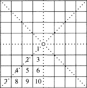
His program therefore assumed that the White King was in one of the ten numbered squares; an arbitrary chessboard can be put into this form by a sequence of at most three reflections. This normalization reduced the disk file to 10×64⁴ or 10×2²⁴ 12-bit records. Thompson further observed that because the Black King cannot be adjacent to the White King, there are only 454 legal board positions for the two Kings in which the White King is in one of the ten squares marked above. Exploiting that fact, his database shrunk to 454×64³ or about 121 million 12-bit records, which fit comfortably on a single (dedicated) disk.

Even though Thompson knew there would be just one copy of his program, he had to squeeze the file onto one disk. Thompson exploited symmetry in data structures to reduce disk space by a factor of eight, which was critical for the success of his entire system. Squeezing space also reduced its run time: decreasing the number of positions examined in the endgame program reduced the time of its learning phase from many months to a few weeks.