Column 14: Heaps

This column is about “heaps”, a data structure that we’ll use to solve two important problems.

Sorting. Heapsort never takes more than O(n log n) time to sort an n-element array, and uses just a few words of extra space.

Priority Queues. Heaps maintain a set of elements under the operations of inserting new elements and extracting the smallest element in the set; each operation requires O(log n) time.

For both problems, heaps are simple to code and computationally efficient.

This column has a bottom-up organization: we start at the details and work up to the big picture. The next two sections describe the heap data structure and two functions to operate on it. The two subsequent sections use those tools to solve the problems mentioned above.

† In other computing contexts, the word “heap” refers to a large segment of memory from which variable-size nodes are allocated; we will ignore that interpretation in this column.

This binary tree is a heap by virtue of two properties. We’ll call the first property order, the value at any node is less than or equal to the values of the node’s children. This implies that the least element of the set is at the root of the tree (12 in the example), but it doesn’t say anything about the relative order of left and right children. The second heap property is shape; the idea is captured by the picture

In words, a binary tree with the shape property has its terminal nodes on at most two levels, with those on the bottom level as far left as possible. There are no “holes” in the tree; if it contains n nodes, no node is at a distance more than log₂ n from the root. We’ll soon see how the two properties together are restrictive enough to allow us to find the minimum element in a set, but lax enough so that we can efficiently reorganize the structure after inserting or deleting an element.

Let’s turn now from the abstract properties of heaps to their implementation. The most common representation of binary trees employs records and pointers. We’ll use an implementation that is suitable only for binary trees with the shape property, but is quite effective for that special case. A 12-element tree with shape is represented in the 12-element array x[1.. 12] as

Notice that heaps use a one-based array; the easiest approach in C is to declare x[n + 1] and waste element x[0]. In this implicit representation of a binary tree, the root is in x[1], its two children are in x[2] and x[3], and so on. The typical functions on the tree are defined as follows.

root = 1
value(i) = x [i]
leftchild(i) = 2*i
rightchild(i) = 2*i+l
parent(i) = i / 2
null(i) = (i < 1) or (i > n)

An n-element implicit tree necessarily has the shape property: it makes no provision for missing elements.

This picture shows a 12-element heap and its implementation as an implicit tree in a 12-element array.

Because the shape property is guaranteed by the representation, from now on the name heap will mean that the value in any node is greater than or equal to the value in its parent. Phrased precisely, the array x[1..n] has the heap property if

∀_2≤i≤n x[i / 2] ≤ x[i]

Recall that the “/” integer division operator rounds down, so 4/2 and 5/2 are both 2. In the next section we will want to talk about the subarray x[l..u] having the heap property (it already has a variant of the shape property); we may mathematically define heap (I, u) as

∀_2l≤i≤u x[i / 2] ≤ x[i]

Placing an arbitrary element in x[n] when x[1..n – 1] is a heap will probably not yield heap(1, n); re-establishing the property is the job of function siftup. Its name describes its strategy: it sifts the new element up the tree as far as it should go, swapping it with its parent along the way. (This section will use the typical heap definition of which way is up: the root of the heap is x[1] at the top of the tree, and therefore x[n] is at the bottom of the array.) The process is illustrated in the following pictures, which (left to right) show the new element 13 being sifted up the heap until it is at its proper position as the right child of the root.

The process continues until the circled node is greater than or equal to its parent (as in this case) or it is at the root of the tree. If the process starts with heap(1, n – 1) true, it leaves heap(1, n) true.

With that intuitive background, let’s write the code. The sifting process calls for a loop, so we start with the loop invariant. In the picture above, the heap property holds everywhere in the tree except between the circled node and its parent. If we let i be the index of the circled node, then we can use the invariant

Click here to view code image

loop
    /* invariant: heap(l, n) except perhaps
            between i and its parent */

Because we originally have heap(1, n – 1), we may initialize the loop by the assignment i = n.

The loop must check whether we have finished yet (either by the circled node being at the top of the heap or greater than or equal to its parent) and, if not, make progress towards termination. The invariant says that the heap property holds everywhere except perhaps between i and its parent. If the test i == 1 is true, then i has no parent and the heap property thus holds everywhere; the loop may therefore terminate. When i does have a parent, we let p be the parent’s index by assigning p = i/2. If x[p]≤x[i] then the heap property holds everywhere, and the loop may terminate.

If, on the other hand, i is out of order with its parent, then we swap x[i] and x[p]. This step is illustrated in the following picture, in which the keys are single letters and node i is circled.

After the swap, all five elements are in the proper order: b <d and b <e because b was originally higher in the heap†, a <b because the test x[p]≤x[i] failed, and a <c by combining a < b and b < c. This gives the heap property everywhere in the array except possibly between p and its parent; we therefore regain the invariant by assigning i = p.

† This important property is unstated in the loop invariant. Don Knuth observes that to be precise, the invariant should be strengthened to “heapi 1, n) holds if i has no parent; otherwise it would hold if x[i] were replaced by x[p], where p is the parent of i”. Similar precision should also be used in the siftdown loop that we will study shortly.

The pieces are assembled in this siftup code, which runs in time proportional to log n because the heap has that many levels.

Click here to view code image

void siftup(n)
         pre n > 0 && heap(l, n-1)
         post heap(l, n)
     i = n
     loop
         /* invariant: heap(l, n) except perhaps
                 between i and its parent */
         if i == 1
             break
         P = i / 2
         if x[p] <= x[i]
             break
         swap(p, i)
         i = P

As in Column 4, the “pre” and “post” lines characterize the function: if the precondition is true before the function is called then the postcondition will be true after the function returns.

We’ll turn now from siftup to siftdown. Assigning a new value to x[1] when x[l..n] is a heap leaves heap(2, n); function siftdown makes heap(l, n) true. It does so by sifting x[1] down the array until either it has no children or it is less than or equal to the children it does have. These pictures show 18 being sifted down the heap until it is finally less than its single child, 19.

When an element is sifted up, it always goes towards the root. Sifting down is more complicated: an out-of-order element is swapped with its lesser child.

The pictures illustrate the invariant of the siftdown loop: the heap property holds everywhere except, possibly, between the circled node and its children.

Click here to view code image

loop
    /* invariant: heap(l, n) except perhaps between
            i and its (0, 1 or 2) children */

The loop is similar to siftup”s. We first check whether i has any children, and terminate the loop if it has none. Now comes the subtle part: if i does have children, then we set the variable c to index the lesser child of i. Finally, we either terminate the loop if x[i]≤x[c], or progress towards the bottom by swapping x[i] and x[c] and assigning i = c.

Click here to view code image

void siftdown(n)
        pre   heap(2, n) && n >= 0
        post  heap(l, n)
    i = 1
    loop
        /* invariant: heap(l, n) except perhaps between
                i and its (0, 1 or 2) children */
        c = 2*i
        if c > n
            break
        /* c is the left child of i */
        if c+1 <= n
            /* c+1 is the right child of i */
            if x[c+l] < x[c]
                C++
        /* c is the lesser child of i */
        if x[i] <= x[c]
            break
        swap(c, i)
        i = c

A case analysis like that done for siftup shows that the swap operation leaves the heap property true everywhere except possibly between c and its children. Like siftup, this function takes time proportional to log n, because it does a fixed amount of work at each level of the heap.

A priority queue manipulates an initially empty set† of elements, which we will call S. The insert function inserts a new element into the set; we can define that more precisely in terms of its pre- and postconditions.

† Because the set can contain multiple copies of the same element, we might be more precise to call it a “multiset” or a “bag”. The union operator is defined so that {2, 3} ∪ {2} = {2, 2, 3}.

Click here to view code image

void insert(t)
        pre   |S| < maxsize
        post  current S = original S ∪ {t}

Function extractmin deletes the smallest element in the set and returns that value in its single parameter t.

Click here to view code image

int extractmin()
        pre   |S| > 0
        post  original S = current S ∪ {result}
                && result = min(original S)

This function could, of course, be modified to yield the maximum element, or any extreme element under a total ordering.

We can specify a C++ class for the job with a template that specifies the type T of elements in the queue:

Click here to view code image

tempiate<class T>
class priqueue {
public:
    priqueue (int maxsize); // init set S to empty
    void insert(T t);       // add t to S
    T extractmin();         // return smallest in S
};

Priority queues are useful in many applications. An operating system may use such a structure to represent a set of tasks; they are inserted in an arbitrary order, and the next task to be executed is extracted:

priqueue<Task> queue;

In discrete event simulation, the elements are times of events; the simulation loop extracts the next event and possibly adds more events to the queue:

priqueue<Event> eventqueue;

In both applications the basic priority queue must be augmented with additional information beyond the elements in the set; we will ignore that “implementation detail” in our discussion, but C++ classes usually handle it gracefully.

Sequential structures such as arrays or linked lists are obvious candidates for implementing priority queues. If the sequence is sorted it is easy to extract the minimum but hard to insert a new element; the situation is reversed for unsorted structures. This table shows the performance of the structures on an n-element set.

Even though binary search can find the position of a new element in O(log n) time, moving the old elements to make way for the new may require O(n) steps. If you’ve forgotten the difference between O(n²) and O(n log n) algorithms, review Section 8.5: when n is one million, the run times of those programs are three hours and one second.

The heap implementation of priority queues provides a middle ground between the two sequential extremes. It represents an n-element set in the array x[l..n] with the heap property, where x is declared in C or C++ as x[maxsize + 1] (we will not use x[0]). We initialize the set to be empty by the assignment n = 0. To insert a new element we increment n and place the new element in x[n]. That gives the situation that siftup was designed to fix: heap(1, n – 1). The insertion code is therefore

void insert(t)
    if n >= maxsize
        /* report error */
    n++
    x[n] = t
    /* heap(1, n-1) */
    siftup(n)
    /* heap(l, n) */

Function extractmin finds the minimum element in the set, deletes it, and restructures the array to have the heap property. Because the array is a heap, the minimum element is in x[1]. The n – 1 elements remaining in the set are now in x[2..n], which has the heap property. We regain heap (I, n) in two steps. We first move x[n] to x[l] and decrement n; the elements of the set are now in x[1..n], and heap(2, n) is true. The second step calls siftdown. The code is straightforward.

int extractmin()
    if n < 1
        /* report error */
    t = x[l]
    x[l] = x[n--]
    /* heap(2, n) */
    siftdown(n)
    /* heap(l, n) */
    return t

Both insert and extractmin require O(log n) time when applied to heaps that contain n elements.

Here is a complete C++ implementation of priority queues:

Click here to view code image

tempiate<class T>
class priqueue {
private:
    int n, maxsize;
    T *x;
    void swap(int i, int j)
    {   T t = x[i]; x[i] = x[j]; x[j] = t; }

public:
    priqueue(int m)
    {   maxsize = m;
        x = new T[maxsize+1];
        n = 0;
    }
    void insert(T t)
    {   int i, p;
        x[++n] = t;
        for (i = n; i > 1 && x[p=i/2] > x[i]; i = p)
            swap(p, i);
    }
    T extractmin()
    {   int i, c;
        T t = x[1];
        x[1] = x[n--];
        for (i = 1; (c = 2*i) <= n; i = c) {
            if (c+1 <= n && x[c+l] < x[c])
                C++;
            if (x[i] <= x[c])
                break;
            swap(c, i);
        }
        return t;
    }
};

This toy interface includes no error checking or destructor, but expresses the guts of the algorithm succinctly. While our pseudocode used a lengthy coding style, this dense code is at the other extreme.

Click here to view code image

tempiate<class T>
void pqsort(T v[], int n)
{   priqueue<T> pq(n);
    int i;
    for (i = 0; i < n; i++)
        pq.insert(v[i]);
    for (i = 0; i < n; i++)
        v[i] = pq.extractmin();
}

The n insert and extractmin operations have a worst-case cost of O(n log n), which is superior to the O(n²) worst-case time of the Quicksorts we built in Column 11. Unfortunately, the array x[0..n] used for heaps requires n + 1 additional words of main memory.

We turn now to the Heapsort, which improves this approach. It uses less code, it uses less space because it doesn’t require the auxiliary array, and it uses less time. For purposes of this algorithm we will assume that siftup and siftdown have been modified to operate on heaps in which the largest element is at the top; that is easy to accomplish by swapping “<” and “>” signs.

The simple algorithm uses two arrays, one for the priority queue and one for the elements to be sorted. Heapsort saves space by using just one. The single implementation array x represents two abstract structures: a heap at the left end and at the right end the sequence of elements, originally in arbitrary order and finally sorted. This picture shows the evolution of the array x; the array is drawn horizontally, while time marches down the vertical axis.

The Heapsort algorithm is a two-stage process: the first n steps build the array into a heap, and the next n steps extract the elements in decreasing order and build the final sorted sequence, right to left.

The first stage builds the heap. Its invariant can be drawn as

This code establishes heap(1, n), by sifting elements to move up front in the array.

Click here to view code image

for i = [2, n]
    /* invariant: heap(1, i-1) */
    siftup(i)
    /* heap(1, i) */

The second stage uses the heap to build the sorted sequence. Its invariant can be drawn as

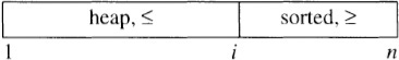
The loop body maintains the invariant in two operations. Because x[1] is the largest among the first i elements, swapping it with x[i] extends the sorted sequence by one element. That swap compromises the heap property, which we regain by sifting down the new top element. The code for the second stage is

Click here to view code image

for (i = n; i >= 2; i--)
    /* heap(1, i)   && sorted(i+1, n) && x[1..i]   <= x[i+1..n] */
    swap(1, i)
    /* heap(2, i-1) && sorted(i, n)   && x[1..i-1] <= x[i..n]   */
    siftdown(i-l)
    /* heap(1, i-1) && sorted(i, n)   && x[1..i-1] <= x[i..n]   */

With the functions we’ve already built, the complete Heapsort algorithm requires just five lines of code.

for i = [2, n]
    siftup(i)
for (i = n; i >= 2; i--)
    swap(1, i )
    siftdown(i-1)

Because the algorithm uses n – 1 siftup and siftdown operations, each of cost at most O(log n), it runs in O(n log n) time, even in the worst case.

Solutions 2 and 3 describe several ways to speed up (and also simplify) the Heap-sort algorithm. Although Heapsort guarantees worst-case O(n log n) performance, for typical input data, the fastest Heapsort is usually slower than the simple Quicksort in Section 11.2.

Correctness. To write code for a loop we first state its invariant precisely; the loop then makes progress towards termination while preserving its invariant. The shape and order properties represent a different kind of invariant: they are invariant properties of the heap data structure. A function that operates on a heap may assume that the properties are true when it starts to work on the structure, and it must in turn make sure that they remain true when it finishes.

Abstraction. Good engineers distinguish between what a component does (the abstraction seen by the user) and how it does it (the implementation inside the black box). This column packages black boxes in two different ways: procedural abstraction and abstract data types.

Procedural Abstraction. You can use a sort function to sort an array without knowing its implementation: you view the sort as a single operation. Functions siftup and siftdown provide a similar level of abstraction: as we built priority queues and Heapsort, we didn’t care how the functions worked, but we knew what they did (fixing an array with the heap property broken at one end or the other). Good engineering allowed us to define these black-box components once, and then use them to assemble two different kinds of tools.

Abstract Data Types. What a data type does is given by its methods and their specifications; how it does it is up to the implementation. We may employ the C++ priqueue class of this column or the C++ IntSet classes of the last column using only their specification to reason about their correctness. Their implementations may, of course, have an impact on the program’s performance.

2. Modify siftdown to have the following specification.

void siftdown(l, u)
        pre   heap(l+1, u)
        post  heap(l, u)

What is the run time of the code? Show how it can be used to construct an n-element heap in O(n) time and thereby a faster Heapsort that also uses less code.

3. Implement Heapsort to run as quickly as possible. How does it compare to the sorting algorithms tabulated in Section 11.3?

4. How might the heap implementation of priority queues be used to solve the following problems? How do your answers change when the inputs are sorted?

a. Construct a Huffman code (such codes are discussed in most books on information theory and many books on data structures).

b. Compute the sum of a large set of floating point numbers.

c. Find the million largest of a billion numbers stored on a file.

d. Merge many small sorted files into one large sorted file (this problem arises in implementing a disk-based merge sort program like that in Section 1.3).

5. The bin packing problem calls for assigning a set of n weights (each between zero and one) to a minimal number of unit-capacity bins. The first-fit heuristic for this problem considers the weights in the sequence in which they are presented, and places each weight into the first bin in which it fits, scanning the bins in increasing order. In his MIT thesis, David Johnson observed that a heap-like structure can implement this heuristic in O(n log n) time. Show how.

6. A common implementation of sequential files on disk has each block point to its successor, which may be any block on the disk. This method requires a constant amount of time to write a block (as the file is originally written), to read the first block in the file, and to read the i^th block, once you have read the i – 1^st block. Reading the i^th block from scratch therefore requires time proportional to i. When Ed McCreight was designing a disk controller at Xerox Palo Alto Research Center, he observed that by adding just one additional pointer per node, you can keep all the other properties, but allow the i block to be read in time proportional to log i. How would you implement that insight? Explain what the algorithm for reading the i^th block has in common with the code in Problem 4.9 for raising a number to the i^th power in time proportional to log i.

7. On some computers the most expensive part of a binary search program is the division by 2 to find the center of the current range. Show how to replace that division with a multiplication by two, assuming that the array to be searched has been constructed properly. Give algorithms for building and searching such a table.

8. What are appropriate implementations for a priority queue that represents integers in the range [0, k), when the average size of the queue is much larger than k?

9. Prove that the simultaneous logarithmic run times of insert and extractmin in the heap implementation of priority queues are within a constant factor of optimal.

10. The basic idea of heaps is familiar to sports fans. Suppose that Brian beat Al and Lynn beat Peter in the semifinals, and that Lynn triumphed over Brian in the championship match. Those results are usually drawn as

Such “tournament trees” are common in tennis tournaments and in post-season playoffs in football, baseball and basketball. Assuming that the results of matches are consistent (an assumption often invalid in athletics), what is the probability that the second-best player is in the championship match? Give an algorithm for “seeding” the players according to their pre-tournament rankings.

11. How are heaps, priority queues and Heapsort implemented in the C++ Standard Template Library?