Installing TensorBoard

Installing TensorBoard can be done with either pip or conda:

pip install tensorboard
conda install tensorboard

TensorBoard can then be started on the command line:

tensorboard --logdir=runs

You can then go to http://[your-machine]:6006, where you’ll see the welcome screen shown in Figure 7-1. We can now send data to the application.

Figure 7-1. TensorBoard

Sending Data to TensorBoard

The module for using TensorBoard with PyTorch is located in torch.utils.tensorboard:

from torch.utils.tensorboard import SummaryWriter
writer = SummaryWriter()
writer.add_scalar('example', 3)

We use the SummaryWriter class to talk to TensorBoard using the standard location for logging output, ./runs, and we can send a scalar by using add_scalar with a tag. Because SummaryWriter works asynchronously, it may take a moment, but you should see TensorBoard update as shown in Figure 7-2.

Figure 7-2. Example data point in TensorBoard

Not very exciting, is it? Let’s write a loop that sends updates from an initial starting point:

import random
value = 10
writer.add_scalar('test_loop', value, 0)
for i in range(1,10000):
  value += random.random() - 0.5
  writer.add_scalar('test_loop', value, i)

By passing where we are in our loop, as shown in Figure 7-3, TensorBoard gives us a plot of the random walk we’re doing from 10. If we run the code again, we’ll see that it has generated a different run inside the display, and we can select on the left side of the web page whether we want to see all our runs or just some in particular.

Figure 7-3. Plotting a random walk in TensorBoard

We can use this to replace our print statements in the training loop. We can also send the model itself to get a representation in TensorBoard!

import torch
import torchvision
from torch.utils.tensorboard import SummaryWriter
from torchvision import datasets, transforms,models

writer = SummaryWriter()
model = models.resnet18(False)
writer.add_graph(model,torch.rand([1,3,224,224]))

def train(model, optimizer, loss_fn, train_data_loader, test_data_loader, epochs=20):
    model = model.train()
    iteration = 0

    for epoch in range(epochs):
        model.train()
        for batch in train_loader:
            optimizer.zero_grad()
            input, target = batch
            output = model(input)
            loss = loss_fn(output, target)
            writer.add_scalar('loss', loss, epoch)
            loss.backward()
            optimizer.step()

        model.eval()
        num_correct = 0
        num_examples = 0
        for batch in val_loader:
            input, target = batch
            output = model(input)
            correct = torch.eq(torch.max(F.softmax(output), dim=1)[1], target).view(-1)
            num_correct += torch.sum(correct).item()
            num_examples += correct.shape[0]
            print("Epoch {}, accuracy = {:.2f}".format(epoch,
                   num_correct / num_examples)
            writer.add_scalar('accuracy', num_correct / num_examples, epoch)
        iterations += 1

When it comes to using add_graph(), we need to send in a tensor to trace through the model as well as the model itself. Once that happens, though, you should see GRAPHS appear in TensorBoard, and as shown in Figure 7-4, clicking the large ResNet block reveals further detail of the model’s structure.

Figure 7-4. Visualizing ResNet

We now have the ability to send accuracy and loss information as well as model structure to TensorBoard. By aggregating multiple runs of accuracy and loss information, we can see whether anything is different in a particular run compared to others, which is a useful clue when trying to work out why a training run produced poor results. We return to TensorBoard shortly, but first let’s look at other features that PyTorch makes available for debugging.

PyTorch Hooks

PyTorch has hooks, which are functions that can be attached to either a tensor or a module on the forward or backward pass. When PyTorch encounters a module with a hook during a pass, it will call the registered hooks. A hook registered on a tensor will be called when its gradient is being calculated.

Hooks are potentially powerful ways of manipulating modules and tensors because you can completely replace the output of what comes into the hook if you so desire. You could change the gradient, mask off activations, replace all the biases in the module, and so on. In this chapter, though, we’re just going to use them as a way of obtaining information about the network as data flows through.

Given a ResNet-18 model, we can attach a forward hook on a particular part of the model by using register_forward_hook:

def print_hook(self, module, input, output):
  print(f"Shape of input is {input.shape}")

model = models.resnet18()
hook_ref  = model.fc.register_forward_hook(print_hook)
model(torch.rand([1,3,224,224]))
hook_ref.remove()
model(torch.rand([1,3,224,224]))

If you run this code you should see text printed out showing the shape of the input to the linear classifier layer of the model. Note that the second time you pass a random tensor through the model, you shouldn’t see the print statement. When we add a hook to a module or tensor, PyTorch returns a reference to that hook. We should always save that reference (here we do it in hook_ref) and then call remove() when we’re finished. If you don’t store the reference, then it will just hang out and take up valuable memory (and potentially waste compute resources during a pass). Backward hooks work in the same way, except you call register_backward_hook() instead.

Of course, if we can print() something, we can certainly send it to TensorBoard! Let’s see how to use both hooks and TensorBoard to get important stats on our layers during training.

Plotting Mean and Standard Deviation

To start, we set up a function that will send the mean and standard deviation of an output layer to TensorBoard:

def send_stats(i, module, input, output):
  writer.add_scalar(f"{i}-mean",output.data.std())
  writer.add_scalar(f"{i}-stddev",output.data.std())

We can’t use this by itself to set up a forward hook, but using the Python function partial(), we can create a series of forward hooks that will attach themselves to a layer with a set i value that will make sure that the correct values are routed to the right graphs in TensorBoard:

from functools import partial

for i,m in enumerate(model.children()):
  m.register_forward_hook(partial(send_stats, i))

Note that we’re using model.children(), which will attach only to each top-level block of the model, so if we have an nn.Sequential() layer (which we will have in a ResNet-based model), we’ll attach a hook to only that block and not one for each individual module within the nn.Sequential list.

If we train our model with our usual training function, we should see the activations start streaming into TensorBoard, as shown in Figure 7-5. You’ll have to switch to wall-clock time within the UI as we’re no longer sending step information back to TensorBoard with the hook (as we’re getting the module information only when the PyTorch hook is called).

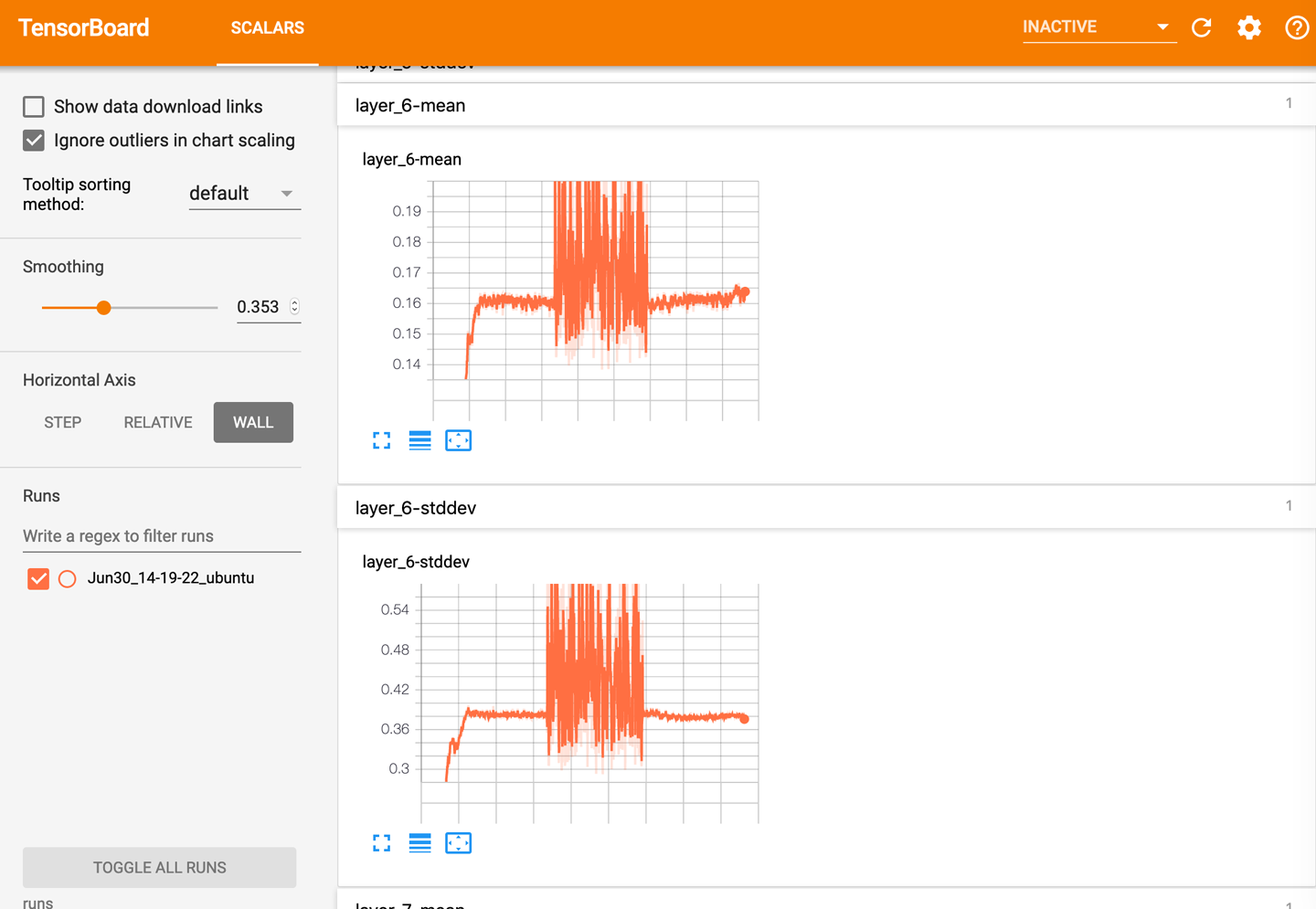
Figure 7-5. Mean and standard deviation of modules in TensorBoard

Now, I mentioned in Chapter 2 that, ideally, layers in a neural network should have a mean of 0 and a standard deviation of 1 to make sure that our calculations don’t run off to infinity or to zero. Have a look at the layers in TensorBoard. Do they look like they’re remaining in that value range? Does the plot sometimes spike and then collapse? If so, that could be a signal that the network is having difficulty training. In Figure 7-5, our mean is close to zero, but our standard deviation is also pretty close to zero as well. If this is happening in many layers of your network, it may be a sign that your activation functions (e.g., ReLU) are not quite suited to your problem domain. It might be worth experimenting with other functions to see if they improve the model’s performance; PyTorch’s LeakyReLU is a good alternative offering similar activations to the standard ReLU but lets more information through, which might help in training.

That about wraps up our look at TensorBoard, but the “Further Reading” will point you to more resources. In the meantime, let’s see how we can get a model to explain how it came to a decision.

Class Activation Mapping

Class activation mapping (CAM) is a technique for visualizing the activations of a network after it has classified an incoming tensor. In image-based classifiers, it’s often shown as a heatmap on top of the original image, as shown in Figure 7-6.

Figure 7-6. Class activation mapping with Casper

From the heatmap, we can get an intuitive idea of how the network reached the decision of Persian Cat from the available ImageNet classes. The activations of the network are at their highest around the face and body of the cat and low elsewhere in the image.

To generate the heatmap, we capture the activations of the final convolutional layer of a network, just before it goes into the Linear layer, as this allows us to see what the combined CNN layers thinks are important as we head into the final mapping from image to classes. Thankfully, with PyTorch’s hook feature, this is fairly straightforward. We wrap up the hook in a class, SaveActivations:

class SaveActivations():
    activations=None
    def __init__(self, m):
      self.hook = m.register_forward_hook(self.hook_fn)
    def hook_fn(self, module, input, output):
      self.features = output.data
    def remove(self):
      self.hook.remove()

We then push our image of Casper through the network (normalizing for ImageNet), apply softmax to turn the output tensor into probabilities, and use torch.topk() as a way of pulling out both the max probability and its index:

import torch
from torchvision import models, transforms
from torch.nn import functional as F

casper = Image.open("casper.jpg")
# Imagenet mean/std

normalize = transforms.Normalize(
   mean=[0.485, 0.456, 0.406],
   std=[0.229, 0.224, 0.225]
)

preprocess = transforms.Compose([
   transforms.Resize((224,224)),
   transforms.ToTensor(),
   normalize
])

display_transform = transforms.Compose([
   transforms.Resize((224,224))])

casper_tensor = preprocess(casper)

model = models.resnet18(pretrained=True)
model.eval()
casper_activations = SaveActivations(model.layer_4)
prediction = model(casper_tensor.unsqueeze(0))
pred_probabilities = F.softmax(prediction).data.squeeze()
casper_activations.remove()
torch.topk(pred_probabilities,1)

If we now access casper_activations.activations, we’ll see that it has been populated by a tensor, which contains the activations of the final convolutional layer we need. We then do this:

fts = sf[0].features[idx]
        prob = np.exp(to_np(log_prob))
        preds = np.argmax(prob[idx])
        fts_np = to_np(fts)
        f2=np.dot(np.rollaxis(fts_np,0,3), prob[idx])
        f2-=f2.min()
        f2/=f2.max()
        f2
plt.imshow(dx)
plt.imshow(scipy.misc.imresize(f2, dx.shape), alpha=0.5, cmap='jet');

This calculates the dot product of the activations from Casper (we index into 0 because of the batching in the first dimension of the input tensor, remember). As mentioned in Chapter 1, PyTorch stores image data in C × H × W format, so we next need to rearrange the dimensions back to H × W × C for displaying the image. We then remove the minimums from the tensor and scale by the maximum to ensure that we’re focusing on only the highest activations in the resulting heatmap (i.e., what speaks to Persian Cat). Finally, we use some matplot magic to display Casper and then the tensor on top, resized and given a standard jet color map. Note that by replacing idx with a different class, you can see the heatmap indicating which activations (if any) are present in the image when classified. So if the model predicts car, you can see which parts of the image were used to make that decision. The second-highest probability for Casper is Angora Rabbit, and we can see from the CAM for that index that it focused on his very fluffy fur!

That wraps up our look into what a model is doing when it makes a decision. Next, we’re going to investigate what a model spends most of its time doing while it’s in a training loop or during inference.

Installing py-spy

There are many ways to generate the stacktraces that can be turned into flame graphs. The one in the previous section was generated using the Linux tool perf, which is a complex and powerful tool. We’ll take a somewhat easier option and use py-spy, a Rust-based stack profiler, to directly generate flame graphs. Install it via pip:

pip install py-spy

You can find the process identifier (PID) of a running process and attach py-spy by using a --pid argument:

py-spy --flame profile.svg --pid 12345

Or you can pass in a Python script, which is how we run it in this chapter. First, let’s run it on a simple Python script:

import torch
import torchvision

def get_model():
    return torchvision.models.resnet18(pretrained=True)

def get_pred(model):
    return model(torch.rand([1,3,224,224]))

model = get_model()

for i in range(1,10000):
    get_pred(model)

Save this as flametest.py and let’s run py-spy on it, sampling 99 times a second and running for 30 seconds:

py-spy -r 99 -d 30 --flame profile.svg -- python t.py

Open the profile.svg file in your browser, and let’s take a look at the resulting graph.

Reading Flame Graphs

Figure 7-8 shows what the graph should look like, roughly speaking (because of sampling, it may not look exactly like this on your machine). The first thing you’ll probably notice is that the graph is going down instead of up. py-spy writes out flame graphs in icicle format, so the stack looks like stalactites instead of the flames of the classic flame graph. I prefer the normal format, but py-spy doesn’t give us the option to change it, and it doesn’t make that much difference.

Figure 7-8. Flame graph on ResNet loading and inference

At a glance, you should see that most of the execution time is spent in various forward() calls, which makes sense because we are making lots of predictions with the model. What about those tiny blocks on the left? If you click them, you should find that the SVG file zooms in as shown in Figure 7-9.

Figure 7-9. Zoomed flame graph

Here, we can see the script setting up the ResNet-18 module and also calling load_state_dict() to load the saved weights from disk (because we called it with pretrained=True). You can click Reset Zoom to go back to the full flame graph. Also, a search bar on the right will highlight matching bars in purple, if you’re trying to hunt down a function. Try it with resnet, and it’ll show you every function call on the stack with resnet in its name. This can be useful for finding functions that aren’t on the stack much or seeing how much that pattern appears in the graph overall.

Play around with the SVG for a bit and see how much CPU time things like BatchNorm and pooling are taking up in this toy example. Next, we’ll look at a way to use flame graphs to find an issue, fix it, and verify it with another flame graph.

Fixing a Slow Transformation

In real-world situations, part of your data pipeline may be causing a slowdown. This is a particular problem if you have a slow transformation, as it will be called many times during a training batch, causing a massive bottleneck in creating your model. Here’s an example transformation pipeline and a data loader:

import torch
import torchvision
from torch import optim
import torch.nn as nn
from torchvision import datasets, transforms, models
import torch.utils.data
from PIL import Image
import numpy as np

device = "cuda:0"
model = models.resnet18(pretrained=True)
model.to(device)


class BadRandom(object):
    def __call__(self, img):
        img_np = np.array(img)
        random = np.random.random_sample(img_np.shape)
        out_np = img_np + random
        out = Image.fromarray(out_np.astype('uint8'), 'RGB')
        return out

    def __repr__(self):
        str = f"{self.__class__.__name__  }"
        return str

train_data_path = "catfish/train"
image_transforms =
torchvision.transforms.Compose(
  [transforms.Resize((224,224)),BadRandom(), transforms.ToTensor()])

We’re not going to run a full training loop; instead, we simulate 10 epochs of just pulling the images from the training data loader:

train_data = torchvision.datasets.ImageFolder(root=train_data_path,
transform=image_transforms)
batch_size=32
train_data_loader = torch.utils.data.DataLoader(train_data,
batch_size=batch_size)

optimizer = optim.Adam(model.parameters(), lr=2e-2)
criterion = nn.CrossEntropyLoss()

def train(model, optimizer, loss_fn,  train_loader, val_loader,
epochs=20, device='cuda:0'):
    model.to(device)
    for epoch in range(epochs):
        print(f"epoch {epoch}")
        model.train()
        for batch in train_loader:
            optimizer.zero_grad()
            ww, target = batch
            ww = ww.to(device)
            target= target.to(device)
            output = model(ww)
            loss = loss_fn(output, target)
            loss.backward()
            optimizer.step()

        model.eval()
        num_correct = 0
        num_examples = 0
        for batch in val_loader:
            input, target = batch
            input = input.to(device)
            target= target.to(device)
            output = model(input)
            correct = torch.eq(torch.max(output, dim=1)[1], target).view(-1)
            num_correct += torch.sum(correct).item()
            num_examples += correct.shape[0]
        print("Epoch {}, accuracy = {:.2f}"
        .format(epoch, num_correct / num_examples))

train(model,optimizer,criterion,
train_data_loader,train_data_loader,epochs=10)

Let’s run that code under py-spy as before:

py-spy -r 99 -d 120 --flame slowloader.svg -- python slowloader.py

If you open the resulting slowloader.svg, you should hopefully see something like Figure 7-10. Although the flame graph is mostly occupied with loading the images and converting them to tensors, we are spending 16.87% of the sampled runtime in applying random noise. Looking at the code, our implementation of BadRandom is applying noise at the PIL stage rather than at the tensor stage, so we’re at the mercy of the imaging library and NumPy rather than PyTorch itself. So our first idea would likely be to rewrite the transform so that it operates on tensors instead of the PIL images. That’s likely to be faster, but not always—and the important thing when making performance changes is always to measure everything.

Figure 7-10. Flame graph with BadRandom

But here’s a curious thing, which has been present all the way through the book, though I’ve not drawn attention to it until now: have you noticed that we pull batches from the data loader and then put those batches onto the GPU? Because the transforms occur as the loader gets batches from the dataset class, those transforms are always going to happen on the CPU. In some cases, that can lead to some crazy lateral thinking. We are applying random noise on every image. What if we could apply random noise on every image at once?

Here’s the bit that might seem mind-bending at first: we’re adding random noise to an image. We can write that as x + y, with x being our image and y our noise. We know that both image and noise are 3D (width, height, channels), so all we’re doing here is matrix multiplication. And in a batch, we’ll be doing this z times. We’re just iterating over each image as we pull them out of the loader. But consider that at the end of the loading process, the images are transformed into tensors, a batch of [z, c, h, w]. Well, couldn’t you just add a random tensor of shape [z, c, h, w] and get the random noise applied that way? Instead of applying the noise in sequence, it happens all at once. We now have a matrix operation, and a very expensive GPU that just happens to be rather good at matrix operations. Try this in Jupyter Notebook to see the difference between CPU and GPU tensor matrix operations:

cpu_t1 = torch.rand(64,3,224,224)
cpu_t2 = torch.rand(64,3,224,224)
%timeit cpu_t1 + cpu_t2
>> 5.39 ms ± 4.29 µs per loop (mean ± std. dev. of 7 runs, 100 loops each)

gpu_t1 = torch.rand(64,3,224,224).to("cuda")
gpu_t2 = torch.rand(64,3,224,224).to("cuda")
%timeit gpu_t1 + gpu_t2
>> 297 µs ± 338 ns per loop (mean ± std. dev. of 7 runs, 10000 loops each)

That’s just under 20 times faster. Instead of performing this transformation in our data loader, we can take it out and perform the matrix operations after we have the entire batch at our disposal:

def add_noise_gpu(tensor, device):
  random_noise = torch_rand_like(tensor).to(device)
  return tensor.add_(random_noise)

In our training loop, add this line after input.to(device):

input = add_noise_gpu(input, device)

Then remove the BadRandom transform from the transform pipeline and test again with py-spy. The new flame graph is shown in Figure 7-11. It’s so fast that it no longer even shows up under our sampling frequency. We’ve just sped up the code by almost 17%! Now, not all standard transforms can be written in a GPU-friendly way, but if it’s possible and the transform is slowing you down, then it’s definitely an option worth considering.

Figure 7-11. Flame graph with GPU-accelerated random noise

Now that we’ve considered compute, it’s time to look at the other elephant in the room: memory, especially memory on the GPU.

Checking Your GPU

Assuming you are using an NVIDIA GPU (check your alternate GPU supplier’s drivers website for their own utilities if you’re using something different), the CUDA installation includes a rather useful command-line tool called nvidia-smi. When run with no arguments, this tool can give you a snapshot of the memory being used on the GPU, and even better, what is using it! Figure 7-12 shows output from running nvidia-smi within the terminal. Within a notebook, you can call out to the utility by using !nvidia-smi.

Figure 7-12. Output from nvidia-smi

This example is taken from my home machine running a 1080 Ti. I’m running a bunch of notebooks, each of which is taking up a chunk of memory, but one is using 4GB! You can get the current PID of a notebook by using os.getpid(). It turns out that the process using the most memory was actually an experimental notebook I was using to test out the GPU transforms in the previous section! You can imagine that with the model, batch data, and data for the forward and backward passes, things get tight memory-wise rather quickly.

In addition, PyTorch will dedicate a chunk of memory to itself and CUDA per process that is around 0.5GB of memory. This means that it’s a better idea to work on one project at a time and not leave Jupyter Notebook running all over the place as I have here (you can use the Kernel menu to shut down the Python process connected to a notebook).

Running nvidia-smi by itself will give you the current snapshot of the GPU’s usage, but you can get continual output by using the -l flag. Here’s an example command that will dump the timestamp, used memory, free memory, total memory, and GPU utilization every 5 seconds:

nvidia-smi --query-gpu=timestamp,
memory.used, memory.free,memory.total,utilization.gpu --format=csv -l 5

If you really think that your GPU is using up more memory than it should be, you can try getting Python’s garbage collector involved. If you have a tensor_to_be_deleted that you no longer need and want it gone from the GPU, then a tip from the bowels of the fast.ai library is to give it a shove with del:

import gc
del tensor_to_be_deleted
gc.collect()

If you’re doing a lot of work inside Jupyter Notebook creating and re-creating models, you may find that deleting some references and invoking the garbage collector by using gc.collect() will claw back some memory. If you’re still having trouble with memory, read on, because there may be an answer to your woes!

Gradient Checkpointing

Despite all the deletion and garbage collection tricks presented in the previous section, you might still find yourself running out of memory. The next thing to do for most applications is to reduce the batch size of data going through a model during the training loop. This will work, but you’re going to increase training time for each epoch, and it’s likely that the model will not be as good as an equivalent one trained with enough memory to handle the larger batch sizes, because you’ll be seeing more of the dataset on every pass. However, we can trade compute against memory for large models in PyTorch by using gradient checkpointing.

One of the problems when dealing with bigger models is that the forward and backward passes create lots of intermediate state, all of which occupy GPU memory. The goal of gradient checkpointing is to reduce the amount of state that may be on the GPU at any one time by segmenting the model. This approach means that you can have between four and ten times the batch size with a nonsegmented model, with that being offset by the training being more compute-intensive. During the forward pass, PyTorch saves the inputs and the parameters to a segment, but doesn’t actually do the forward pass itself. During the backward pass, these are retrieved by PyTorch, and the forward pass is computed for that segment. The intermediate values are passed onto the next segment, but those have to be performed on only a segment-by-segment basis.

Chopping up a model into these segments is handled by torch.utils.checkpoint.checkpoint_sequential(). It works on nn.Sequential layers or generated lists of layers, with the proviso that they need to be in sequence of how they occur in the model. Here’s how it would work on the features module in AlexNet:

from torch.utils.checkpoint import checkpoint_sequential
import torch.nn as nn

class CheckpointedAlexNet(nn.Module):

    def __init__(self, num_classes=1000, chunks=2):
        super(CheckpointedAlexNet, self).__init__()
        self.features = nn.Sequential(
            nn.Conv2d(3, 64, kernel_size=11, stride=4, padding=2),
            nn.ReLU(inplace=True),
            nn.MaxPool2d(kernel_size=3, stride=2),
            nn.Conv2d(64, 192, kernel_size=5, padding=2),
            nn.ReLU(inplace=True),
            nn.MaxPool2d(kernel_size=3, stride=2),
            nn.Conv2d(192, 384, kernel_size=3, padding=1),
            nn.ReLU(inplace=True),
            nn.Conv2d(384, 256, kernel_size=3, padding=1),
            nn.ReLU(inplace=True),
            nn.Conv2d(256, 256, kernel_size=3, padding=1),
            nn.ReLU(inplace=True),
            nn.MaxPool2d(kernel_size=3, stride=2),
        )
        self.avgpool = nn.AdaptiveAvgPool2d((6, 6))
        self.classifier = nn.Sequential(
            nn.Dropout(),
            nn.Linear(256 * 6 * 6, 4096),
            nn.ReLU(inplace=True),
            nn.Dropout(),
            nn.Linear(4096, 4096),
            nn.ReLU(inplace=True),
            nn.Linear(4096, num_classes),
        )

    def forward(self, x):
        x = checkpoint_sequential(self.features, chunks, x)
        x = self.avgpool(x)
        x = x.view(x.size(0), 256 * 6 * 6)
        x = self.classifier(x)
        return x

As you can see, not much is different here, making checkpointing an easy addition to models when required. We’ve added a chunks parameter to the new version of the model, with the default being to split it into two segments. All we then need to do is make a call to checkpoint_sequential with the features module, the number of segments, and our inputs. And that’s it!

One slight kink in checkpointing is that it doesn’t behave well with BatchNorm or Dropout layers because of how they interact with the forward pass. To work around that, you can just checkpoint parts of the model before and after those layers. In our CheckpointedAlexNet, we could perhaps break the classifier module into two parts: one containing the Dropout layers that are uncheckpointed, and a final nn.Sequential module containing our Linear layers that we could checkpoint in the same way we did with features.

If you find yourself with diminishing batch sizes in order to get a model to run, consider checkpointing before you ask for a larger GPU!