Chapter 3. Convolutional Neural Networks
After experimenting with the fully connected neural networks in Chapter 2, you probably noticed a few things. If you attempted to add more layers or vastly increase the number of parameters, you almost certainly ran out of memory on your GPU. In addition, it took a while to train to anything resembling somewhat decent accuracy, and even that wasn’t much to shout about, especially considering the hype surrounding deep learning. What’s going on?
It’s true that a fully connected or (feed-forward) network can function as a universal approximator, but the theory doesn’t say how long it’ll take you to train it to become that approximation to the function you’re really after. But we can do better, especially with images. In this chapter, you’ll learn about convolutional neural networks (CNNs) and how they form the backbone of the most accurate image classifiers around today (we take a look at a couple of them in some detail along the way). We build up a new convolutional-based architecture for our fish versus cat application and show that it is quicker to train and more accurate than what we were doing in the previous chapter. Let’s get started!
Our First Convolutional Model
This time around, I’m going to share the final model architecture first, and then discuss all the new pieces. And as I mentioned in Chapter 2, the training method we created is independent of the model, so you can go ahead and test this model out first and then come back for the explanation!
classCNNNet(nn.Module):def__init__(self,num_classes=2):super(CNNNet,self).__init__()self.features=nn.Sequential(nn.Conv2d(3,64,kernel_size=11,stride=4,padding=2),nn.ReLU(),nn.MaxPool2d(kernel_size=3,stride=2),nn.Conv2d(64,192,kernel_size=5,padding=2),nn.ReLU(),nn.MaxPool2d(kernel_size=3,stride=2),nn.Conv2d(192,384,kernel_size=3,padding=1),nn.ReLU(),nn.Conv2d(384,256,kernel_size=3,padding=1),nn.ReLU(),nn.Conv2d(256,256,kernel_size=3,padding=1),nn.ReLU(),nn.MaxPool2d(kernel_size=3,stride=2),)self.avgpool=nn.AdaptiveAvgPool2d((6,6))self.classifier=nn.Sequential(nn.Dropout(),nn.Linear(256*6*6,4096),nn.ReLU(),nn.Dropout(),nn.Linear(4096,4096),nn.ReLU(),nn.Linear(4096,num_classes))defforward(self,x):x=self.features(x)x=self.avgpool(x)x=torch.flatten(x,1)x=self.classifier(x)returnx
The first thing to notice is the use of nn.Sequential(). This allows us to create a chain of layers. When we use one of these chains in forward(), the input goes through each element of the array of layers in succession. You can use this to break your model into more logical arrangements. In this network, we have two chains: the features block and the classifier. Let’s take a look at the new layers we’re introducing, starting with Conv2d.
Convolutions
The Conv2d layer is a 2D convolution. If we have a grayscale image, it consists of an array, x pixels wide and y pixels high, with each entry having a value that indicates whether it’s black or white or somewhere in between (we assume an 8-bit image, so each value can vary from 0 to 255). For this example we look at a small, square image that’s 4 pixels high and wide:
Next we introduce something called a filter, or convolutional kernel. This is another matrix, most likely smaller, which we will drag across our image. Here’s our 2 × 2 filter:
To produce our output, we take the smaller filter and pass it over the original input, like a magnifying glass over a piece of paper. Starting from the top left, our first calculation is as follows:
And all we do is multiply each element in the matrix by its corresponding member in the other matrix and sum the result: (10 × 1) + (11 × 0) + (2 × 1) + (123 × 0) = 12. Having done that, we move the filter across and begin again. But how much should we move the filter? In this case, we move the filter across by 2, meaning that our second calculation is:
This gives us an output of 13. We now move our filter down and back to the left and repeat the process, giving us this final result (or feature map):
In Figure 3-1, you can see how this works graphically, with a 3 × 3 kernel being dragged across a 4 × 4 tensor and producing a 2 × 2 output (though each segment is based on nine elements instead of the four in our first example).

Figure 3-1. How a 3 × 3 kernel operates across a 4 × 4 input
A convolutional layer will have many of these filters, the values of which are filled in by the training of the network, and all the filters in the layer share the same bias values. Let’s go back to how we’re invoking the Conv2d layer and see some of the other options that we can set:
nn.Conv2d(in_channels,out_channels,kernel_size,stride,padding)
The in_channels is the number of input channels we’ll be receiving in the layer. At the beginning of the network, we’re taking in the RGB image as input, so the number of input channels is three. out_channels is, unsurprisingly, the number of output channels, which corresponds to the number of filters in our conv layer. Next is kernel_size, which describes the height and width of our filter.1 This can be a single scalar specifying a square (e.g., in the first conv layer, we’re setting up an 11 × 11 filter), or you can use a tuple (such as (3,5) for a 3 × 5 filter).
The next two parameters seem harmless enough, but they can have big effects on the downstream layers of your network, and even what that particular layer ends up looking at. stride indicates how many steps across the input we move when we adjust the filter to a new position. In our example, we end up with a stride of 2, which has the effect of making a feature map that is half the size of the input. But we could have also moved with a stride of 1, which would give us a feature map output of 4 × 4, the same size of the input. We can also pass in a tuple (a,b) that would allow us to move a across and b down on each step. Now, you might be wondering, what happens when it gets to the end? Let’s take a look. If we drag our filter along with a stride of 1, we eventually get to this point:
We don’t have enough elements in our input to do a full convolution. So what happens? This is where the padding parameter comes in. If we give a padding value of 1, our input looks a bit like this:
Now when we get to the edge, our values covered by the filter are as follows:
If you don’t set padding, any edge cases that PyTorch encounters in the last columns of the input are simply thrown away. It’s up to you to set padding appropriately. Just as with stride and kernel_size, you can also pass in a tuple for height × weight padding instead of a single number that pads the same in both directions.
That’s what the Conv2d layers are doing in our model. But what about those MaxPool2d layers?
Pooling
In conjunction with the convolution layers, you will often see pooling layers. These layers reduce the resolution of the network from the previous input layer, which gives us fewer parameters in lower layers. This compression results in faster computation for a start, and it helps prevent overfitting in the network.
In our model, we’re using MaxPool2d with a kernel size of 3 and a stride of 2. Let’s have a look at how that works with an example. Here’s a 5 × 3 input:
Using the kernel size of 3 × 3 and a stride of 2, we get two 3 × 3 tensors from the pooling:
In MaxPool we take the maximum value from each of these tensors, giving us an output tensor of [6,9]. Just as in the convolutional layers, there’s a padding option to MaxPool that creates a border of zero values around the tensor in case the stride goes outside the tensor window.
As you can imagine, you can pool with other functions aside from taking the maximum value from a kernel. A popular alternative is to take the average of the tensor values, which allows all of the tensor data to contribute to the pool instead of just one value in the max case (and if you think about an image, you can imagine that you might want to consider the nearest neighbors of a pixel). Also, PyTorch provides AdaptiveMaxPool and AdaptiveAvgPool layers, which work independently of the incoming input tensor’s dimensions (we have an AdaptiveAvgPool in our model, for example). I recommend using these in model architectures that you construct over the standard MaxPool or AvgPool layers, because they allow you to create architectures that can work with different input dimensions; this is handy when working with disparate datasets.
We have one more new component to talk about, one that is incredibly simple yet important for training.
Dropout
One recurring issue with neural networks is their tendency to overfit to training data, and a large amount of ongoing work is done in the deep learning world to identify approaches that allow networks to learn and generalize to nontraining data without simply learning how to just respond to the training inputs. The Dropout layer is a devilishly simple way of doing this that has the benefit of being easy to understand and effective: what if we just don’t train a random bunch of nodes within the network during a training cycle? Because they won’t be updated, they won’t have the chance to overfit to the input data, and because it’s random, each training cycle will ignore a different selection of the input, which should help generalization even further.
By default, the Dropout layers in our example CNN network are initialized with 0.5, meaning that 50% of the input tensor is randomly zeroed out. If you want to change that to 20%, add the p parameter to the initialization call: Dropout(p=0.2).
Note
Dropout should take place only during training. If it was happening during inference time, you’d lose a chunk of your network’s reasoning power, which is not what we want! Thankfully, PyTorch’s implementation of Dropout works out which mode you’re running in and passes all the data through the Dropout layer at inference time.
Having looked at our little CNN model and examined the layer types in depth, let’s take a look at other models that have been made in the past ten years.
History of CNN Architectures
Although CNN models have been around for decades (LeNet-5 was used for digit recognition on check in the late 1990s, for example), it wasn’t until GPUs became widely available that deep CNN networks became practical. Even then, it has been only seven years since deep learning networks started to overwhelm all other existing approaches in image classification. In this section, we take a little journey back through the last few years to talk about some milestones in CNN-based learning and investigate some new techniques along the way.
AlexNet
AlexNet was, in many ways, the architecture that changed everything. It was released in 2012 and destroyed all other entries in that year’s ImageNet competition with a top-5 error rate of 15.3% (the second place entry had a top-5 error of 26.2%, just to give you an idea of how much better it was than other state-of-the-art methods). AlexNet was one of the first architectures to introduce the concepts of MaxPool and Dropout, and even popularize the then less-well-known ReLU activation function. It was one of the first architectures to demonstrate that many layers were possible and efficient to train on a GPU. Although it’s not state of the art anymore, it remains an important milestone in deep learning history.
What does the AlexNet architecture look like? Aha, well, it’s time to let you in on a little secret. The network we’ve been using in this chapter so far? It’s AlexNet. Surprise! That’s why we used the standard MaxPool2d instead of AdaptiveMaxPool2d, to match the original AlexNet definition.
Inception/GoogLeNet
Let’s skip ahead to the winner of the 2014 ImageNet competition. The GoogLeNet architecture introduced the Inception module that addressed some of the deficiencies of AlexNet. In that network, the kernels of the convolutional layers are fixed at a certain resolution. We might expect that an image will have details that are important at both the macro- and microscale. It may be easier to determine whether an object is a car with a large kernel, but to determine whether it’s an SUV or a hatchback may require a smaller kernel. And to determine the model, we might need an even smaller kernel to make out details such as logos and insignias.
The Inception network instead runs a series of convolutions of different sizes all on the same input, and concatenates all of the filters together to pass on to the next layer. Before it does any of those, though, it does a 1 × 1 convolution as a bottleneck that compresses the input tensor, meaning that the 3 × 3 and 5 × 5 kernels operate on a fewer number of filters than they would if the 1 × 1 convolution wasn’t present. You can see an Inception module illustrated in Figure 3-2.

Figure 3-2. An Inception module
The original GoogLeNet architecture uses nine of these modules stacked on top of each other, forming a deep network. Despite the depth, it uses fewer parameters overall than AlexNet while delivering a human-like performance of an 6.67% top-5 error rate.
VGG
The second-place entry in 2014’s ImageNet was from the University of Oxford—the Visual Geometry Group (VGG) network. In contrast to GoogLeNet, VGG is a simpler stack of convolutional layers. Coming in various configurations of longer stacks of convolutional filters combined with two large hidden linear layers before the final classification layer, it shows off the power of simple deep architectures (scoring an 8.8% top-5 error in its VGG-16 configuration). Figure 3-3 shows the layers of the VGG-16 from end to end.
The downside of the VGG approach is that the final fully connected layers make the network balloon to a large size, weighing in at 138 million parameters in comparison with GoogLeNet’s 7 million. Having said that, the VGG network is still quite popular in the deep learning world despite its huge size, as it’s easy to reason about because of its simpler construction and the early availability of trained weights. You’ll often see it used in style transfer applications (e.g., turning a photo into a Van Gogh painting) as its combination of convolutional filters do appear to capture that sort of information in a way that’s easier to observe than the more complex networks.

Figure 3-3. VGG-16
ResNet
A year later, Microsoft’s ResNet architecture won the ImageNet 2015 competition with a top-5 score of 4.49% in its ResNet-152 variant and 3.57% in an ensemble model (essentially beyond human ability at this point). The innovation that ResNet brought was an improvement on the Inception-style stacking bundle of layers approach, wherein each bundle performed the usual CNN operations but also added the incoming input to the output of the block, as shown in Figure 3-4.
The advantage of this set up is that each block passes through the original input to the next layer, allowing the “signal” of the training data to traverse through deeper networks than possible in either VGG or Inception. (This loss of weight changes in deep networks is known as a vanishing gradient because of the gradient changes in backpropagation tending to zero during the training process.)
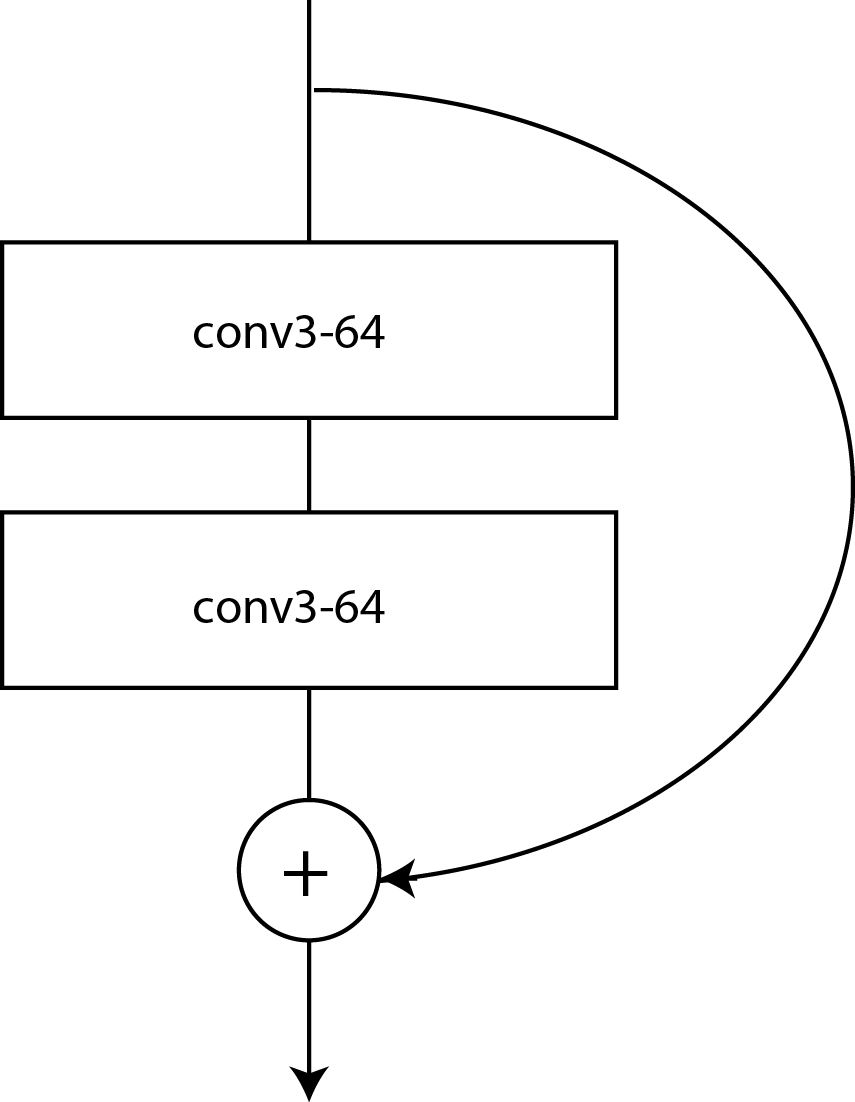
Figure 3-4. A ResNet block
Other Architectures Are Available!
Since 2015 or so, plenty of other architectures have incrementally improved the accuracy on ImageNet, such as DenseNet (an extension of the ResNet idea that allows for the construction of 1,000-layer monster architectures), but also a lot of work has gone into creating architectures such as SqueezeNet and MobileNet, which offer reasonable accuracy but are tiny compared to architectures such as VGG, ResNet, or Inception.
Another big area of research is getting neural networks to start designing neural networks themselves. The most successful attempt so far is, of course, from Google, whose AutoML system generated an architecture called NASNet that has a top-5 error rate of 3.8% on ImageNet, which is state of the art as I type this at the start of 2019 (along with another autogenerated architecture from Google called PNAS). In fact, the organizers of the ImageNet competition have decided to call a halt to further competitions in this space because the architectures have already gone beyond human levels of ability.
That brings us to the state of the art as of the time this book goes to press, so let’s take a look at how we can use these models instead of defining our own.
Using Pretrained Models in PyTorch
Obviously, having to define a model each time you want to use one would be a chore, especially once you move away from AlexNet, so PyTorch provides many of the most popular models by default in the torchvision library. For AlexNet, all you need to do is this:
importtorchvision.modelsasmodelsalexnet=models.alexnet(num_classes=2)
Definitions for VGG, ResNet, Inception, DenseNet, and SqueezeNet variants are also available. That gives you the model definition, but you can also go a step further and call models.alexnet(pretrained=True) to download a pretrained set of weights for AlexNet, allowing you to use it immediately for classification with no extra training. (But as you’ll see in the next chapter, you will likely want to do some additional training to improve the accuracy on your particular dataset.)
Having said that, there is something to be said for building the models yourself at least once to get a feel for how they fit together. It’s a good way to get some practice building model architectures within PyTorch, and of course you can compare with the provided models to make sure that what you come up with matches the actual definition. But how do you find out what that structure is?
Examining a Model’s Structure
If you’re curious about how one of these models is constructed, there’s an easy way to get PyTorch to help you out. As an example, here’s a look at the entire ResNet-18 architecture, which we get by simply calling the following:
(model)ResNet((conv1):Conv2d(3,64,kernel_size=(7,7),stride=(2,2),padding=(3,3),bias=False)(bn1):BatchNorm2d(64,eps=1e-05,momentum=0.1,affine=True,track_running_stats=True)(relu):ReLU(inplace)(maxpool):MaxPool2d(kernel_size=3,stride=2,padding=1,dilation=1,ceil_mode=False)(layer1):Sequential((0):BasicBlock((conv1):Conv2d(64,64,kernel_size=(3,3),stride=(1,1),padding=(1,1),bias=False)(bn1):BatchNorm2d(64,eps=1e-05,momentum=0.1,affine=True,track_running_stats=True)(relu):ReLU(inplace)(conv2):Conv2d(64,64,kernel_size=(3,3),stride=(1,1),padding=(1,1),bias=False)(bn2):BatchNorm2d(64,eps=1e-05,momentum=0.1,affine=True,track_running_stats=True))(1):BasicBlock((conv1):Conv2d(64,64,kernel_size=(3,3),stride=(1,1),padding=(1,1),bias=False)(bn1):BatchNorm2d(64,eps=1e-05,momentum=0.1,affine=True,track_running_stats=True)(relu):ReLU(inplace)(conv2):Conv2d(64,64,kernel_size=(3,3),stride=(1,1),padding=(1,1),bias=False)(bn2):BatchNorm2d(64,eps=1e-05,momentum=0.1,affine=True,track_running_stats=True)))(layer2):Sequential((0):BasicBlock((conv1):Conv2d(64,128,kernel_size=(3,3),stride=(2,2),padding=(1,1),bias=False)(bn1):BatchNorm2d(128,eps=1e-05,momentum=0.1,affine=True,track_running_stats=True)(relu):ReLU(inplace)(conv2):Conv2d(128,128,kernel_size=(3,3),stride=(1,1),padding=(1,1),bias=False)(bn2):BatchNorm2d(128,eps=1e-05,momentum=0.1,affine=True,track_running_stats=True)(downsample):Sequential((0):Conv2d(64,128,kernel_size=(1,1),stride=(2,2),bias=False)(1):BatchNorm2d(128,eps=1e-05,momentum=0.1,affine=True,track_running_stats=True)))(1):BasicBlock((conv1):Conv2d(128,128,kernel_size=(3,3),stride=(1,1),padding=(1,1),bias=False)(bn1):BatchNorm2d(128,eps=1e-05,momentum=0.1,affine=True,track_running_stats=True)(relu):ReLU(inplace)(conv2):Conv2d(128,128,kernel_size=(3,3),stride=(1,1),padding=(1,1),bias=False)(bn2):BatchNorm2d(128,eps=1e-05,momentum=0.1,affine=True,track_running_stats=True)))(layer3):Sequential((0):BasicBlock((conv1):Conv2d(128,256,kernel_size=(3,3),stride=(2,2),padding=(1,1),bias=False)(bn1):BatchNorm2d(256,eps=1e-05,momentum=0.1,affine=True,track_running_stats=True)(relu):ReLU(inplace)(conv2):Conv2d(256,256,kernel_size=(3,3),stride=(1,1),padding=(1,1),bias=False)(bn2):BatchNorm2d(256,eps=1e-05,momentum=0.1,affine=True,track_running_stats=True)(downsample):Sequential((0):Conv2d(128,256,kernel_size=(1,1),stride=(2,2),bias=False)(1):BatchNorm2d(256,eps=1e-05,momentum=0.1,affine=True,track_running_stats=True)))(1):BasicBlock((conv1):Conv2d(256,256,kernel_size=(3,3),stride=(1,1),padding=(1,1),bias=False)(bn1):BatchNorm2d(256,eps=1e-05,momentum=0.1,affine=True,track_running_stats=True)(relu):ReLU(inplace)(conv2):Conv2d(256,256,kernel_size=(3,3),stride=(1,1),padding=(1,1),bias=False)(bn2):BatchNorm2d(256,eps=1e-05,momentum=0.1,affine=True,track_running_stats=True)))(layer4):Sequential((0):BasicBlock((conv1):Conv2d(256,512,kernel_size=(3,3),stride=(2,2),padding=(1,1),bias=False)(bn1):BatchNorm2d(512,eps=1e-05,momentum=0.1,affine=True,track_running_stats=True)(relu):ReLU(inplace)(conv2):Conv2d(512,512,kernel_size=(3,3),stride=(1,1),padding=(1,1),bias=False)(bn2):BatchNorm2d(512,eps=1e-05,momentum=0.1,affine=True,track_running_stats=True)(downsample):Sequential((0):Conv2d(256,512,kernel_size=(1,1),stride=(2,2),bias=False)(1):BatchNorm2d(512,eps=1e-05,momentum=0.1,affine=True,track_running_stats=True)))(1):BasicBlock((conv1):Conv2d(512,512,kernel_size=(3,3),stride=(1,1),padding=(1,1),bias=False)(bn1):BatchNorm2d(512,eps=1e-05,momentum=0.1,affine=True,track_running_stats=True)(relu):ReLU(inplace)(conv2):Conv2d(512,512,kernel_size=(3,3),stride=(1,1),padding=(1,1),bias=False)(bn2):BatchNorm2d(512,eps=1e-05,momentum=0.1,affine=True,track_running_stats=True)))(avgpool):AdaptiveAvgPool2d(output_size=(1,1))(fc):Linear(in_features=512,out_features=1000,bias=True))
There’s almost nothing here you haven’t already seen in this chapter, with the exception of BatchNorm2d. Let’s have a look at what that does in one of those layers.
BatchNorm
BatchNorm, short for batch normalization, is a simple layer that has one task in life: using two learned parameters (meaning that it will be trained along with the rest of the network) to try to ensure that each minibatch that goes through the network has a mean centered around zero with a variance of 1. You might ask why we need to do this when we’ve already normalized our input by using the transform chain in Chapter 2. For smaller networks, BatchNorm is indeed less useful, but as they get larger, the effect of any layer on another, say 20 layers down, can be vast because of repeated multiplication, and you may end up with either vanishing or exploding gradients, both of which are fatal to the training process. The BatchNorm layers make sure that even if you use a model such as ResNet-152, the multiplications inside your network don’t get out of hand.
You might be wondering: if we have BatchNorm in our network, why are we normalizing the input at all in the training loop’s transformation chain? After all, shouldn’t BatchNorm do the work for us? And the answer here is yes, you could do that! But it’ll take longer for the network to learn how to get the inputs under control, as they’ll have to discover the initial transform themselves, which will make training longer.
I recommend that you instantiate all of the architectures we’ve talked about so far and use print(model) to see which layers they use and in what order operations happen. After that, there’s another key question: which of these architectures should I use?
Which Model Should You Use?
The unhelpful answer is, whichever one works best for you, naturally! But let’s dig in a little. First, although I suggest that you try the NASNet and PNAS architectures at the moment, I wouldn’t wholeheartedly recommend them, despite their impressive results on ImageNet. They can be surprisingly memory-hungry in operation, and the transfer learning technique, which you learn about in Chapter 4, is not quite as effective compared to the human-built architectures including ResNet.
I suggest that you have a look around the image-based competitions on Kaggle, a website that runs hundreds of data science competitions, and see what the winning entries are using. More than likely you’ll end up seeing a bunch of ResNet-based ensembles. Personally, I like and use the ResNet architectures over and above any of the others listed here, first because they offer good accuracy, and second because it’s easy to start out experimenting with a ResNet-34 model for fast iteration and then move to larger ResNets (and more realistically, an ensemble of different ResNet architectures, just as Microsoft used in their ImageNet win in 2015) once I feel I have something promising.
Before we end the chapter, I have some breaking news concerning downloading pretrained models.
One-Stop Shopping for Models: PyTorch Hub
A recent announcement in the PyTorch world provides an additional route to get models: PyTorch Hub. This is supposed to become a central location for obtaining any published model in the future, whether it’s for operating on images, text, audio, video, or any other type of data. To obtain a model in this fashion, you use the torch.hub module:
model=torch.hub.load('pytorch/vision','resnet50',pretrained=True)
The first parameter points to a GitHub owner and repository (with an optional tag/branch identifier in the string as well); the second is the model requested (in this case, resnet50); and finally, the third indicates whether to download pretrained weights. You can also use torch.hub.list('pytorch/vision') to discover all the models inside that repository that are available to download.
PyTorch Hub is brand new as of mid-2019, so there aren’t a huge number of models available as I write this, but I expect it to become a popular way to distribute and download models by the end of the year. All the models in this chapter can be loaded through the pytorch/vision repo in PytorchHub, so feel free to use this loading process instead of torchvision.models.
Conclusion
In this chapter, you’ve taken a quick walk-through of how CNN-based neural networks work, including features such as Dropout, MaxPool, and BatchNorm. You’ve also looked at the most popular architectures used in industry today. Before moving on to the next chapter, play with the architectures we’ve been talking about and see how they compare. (Don’t forget, you don’t need to train them! Just download the weights and test the model.)
We’re going to close out our look at computer vision by using these pretrained models as a starting point for a custom solution for our cats versus fish problem that uses transfer learning.
Further Reading
-
AlexNet: “ImageNet Classification with Deep Convolutional Neural Networks” by Alex Krizhevsky et al. (2012)
-
VGG: “Very Deep Convolutional Networks for Large-Scale Image Recognition” by Karen Simonyan and Andrew Zisserman (2014)
-
Inception: “Going Deeper with Convolutions” by Christian Szegedy et al. (2014)
-
ResNet: “Deep Residual Learning for Image Recognition” by Kaiming He et al. (2015)
-
NASNet: “Learning Transferable Architectures for Scalable Image Recognition” by Barret Zoph et al. (2017)
1 Kernel and filter tend to be used interchangeably in the literature. If you have experience in graphics processing, kernel is probably more familiar to you, but I prefer filter.