6
Functions
As you begin to take on data science projects, you will find that the tasks you perform will involve multiple different instructions (lines of code). Moreover, you will often want to be able to repeat these tasks (both within and across projects). For example, there are many steps involved in computing summary statistics for some data, and you may want to repeat this analysis for different variables in a data set or perform the same type of analysis across two different data sets. Planning out and writing your code will be notably easier if can you group together the lines of code associated with each overarching task into a single step.
Functions represent a way for you to add a label to a group of instructions. Thinking about the tasks you need to perform (rather than the individual lines of code you need to write) provides a useful abstraction in the way you think about your programming. It will help you hide the details and generalize your work, allowing you to better reason about it. Instead of thinking about the many lines of code involved in each task, you can think about the task itself (e.g., compute_summary_ stats()). In addition to helping you better reason about your code, labeling groups of instructions will allow you to save time by reusing your code in different contexts—repeating the task without rewriting the individual instructions.
This chapter explores how to use functions in R to perform advanced capabilities and create code that is flexible for analyzing multiple data sets. After considering a function in a general sense, it discusses using built-in R functions, accessing additional functions by loading R packages, and writing your own functions.
6.1 What Is a Function?
In a broad sense, a function is a named sequence of instructions (lines of code) that you may want to perform one or more times throughout a program. Functions provide a way of encapsulating multiple instructions into a single “unit” that can be used in a variety of contexts. So, rather than needing to repeatedly write down all the individual instructions for drawing a chart for every one of your variables, you can define a make_chart() function once and then just call (execute) that function when you want to perform those steps.
In addition to grouping instructions, functions in programming languages like R tend to follow the mathematical definition of functions, which is a set of operations (instructions!) that are performed on some inputs and lead to some outputs. Function inputs are called arguments (also referred to as parameters); specifying an argument for a function is called passing the argument into the function (like passing a football). A function then returns an output to use. For example, imagine a function that can determine the largest number in a set of numbers—that function’s input would be the set of numbers, and the output would be the largest number in the set.
Grouping instructions into reusable functions is helpful throughout the data science process, including areas such as the following:
Data management: You can group instructions for loading and organizing data so they can be applied to multiple data sets.
Data analysis: You can store the steps for calculating a metric of interest so that you can repeat your analysis for multiple variables.
Data visualization: You can define a process for creating graphics with a particular structure and style so that you can generate consistent reports.
6.1.1 R Function Syntax
R functions are referred to by name (technically, they are values like any other variable). As in many programming languages, you call a function by writing the name of the function followed immediately (no space) by parentheses (). Inside the parentheses, you put the arguments (inputs) to the function separated by commas (,). Thus, computer functions look just like multi-variable mathematical functions, but with names longer than f(). Here are a few examples of using functions that are included in the R language:
# Call the print() function, passing it "Hello world" as an argument
print("Hello world")
# [1] "Hello world"

# Call the sqrt() function, passing it 25 as an argument
sqrt (25) # returns 5 (square root of 25)

# Call the min() function, passing it 1, 6/8, and 4/3 as arguments
# This is an example of a function that takes multiple arguments
min(1, 6 / 8, 4 / 3) # returns 0.75 (6/8 is the smallest value)
Remember
In this text, we always include empty parentheses () when referring to a function by name to help distinguish between variables that hold functions and variables that hold values (e.g., add_values() versus my_value). This does not mean that the function takes no arguments; instead, it is just a useful shorthand for indicating that a variable holds a function (not a value).
If you call any of these functions interactively, R will display the returned value (the output) in the console. However, the computer is not able to “read” what is written in the console—that’s for humans to view! If you want the computer to be able to use a returned value, you will need to give that value a name so that the computer can refer to it. That is, you need to store the returned value in a variable:
# Store the minimum value of a vector in the variable `smallest_number`
smallest_number <- min(1, 6 / 8, 4 / 3)

# You can then use the variable as usual, such as for a comparison
min_is_greater_than_one <- smallest_number > 1 # returns FALSE

# You can also use functions inline with other operations
phi <- .5 + sqrt(5) / 2 # returns 1.618034

# You can pass the result of a function as an argument to another function
# Watch out for where the parentheses close!
print(min(1.5, sqrt(3)))
# [1] 1.5
In the last example, the resulting value of the “inner” function function—sqrt()—is immediately used as an argument. Because that value is used immediately, you don’t have to assign it a separate variable name. Consequently, it is known as an anonymous variable.
6.2 Built-in R Functions
As you have likely noticed, R comes with a variety of functions that are built into the language (also referred to as “base” R functions). The preceding example used the print() function to print a value to the console, the min() function to find the smallest number among the arguments, and the sqrt() function to take the square root of a number. Table 6.1 provides a very limited list of functions you might experiment with (or see a few more from Quick-R1).
Table 6.1 Examples and descriptions of frequently used R functions
Function Name |
Description |
Example |
|
Calculates the sum of all input values |
|
|
Rounds the first argument to the given number of digits |
|
|
Returns the characters in uppercase |
|
|
Concatenates (combines) characters into one value |
|
|
Counts the number of characters in a string (including spaces and punctuation) |
|
|
Concatenates (combines) multiple items into a vector (see Chapter 7) |
|
|
Returns a sequence of numbers from |
|
1Quick-R: Built-in Functions: http://www.statmethods.net/management/functions.html
To learn more about any individual function, you can look it up in the R documentation by using ?FUNCTION_NAME as described in Chapter 5.
Tip
Part of learning any programming language is identifying which functions are available in that language and understanding how to use them. Thus, you should look around and become familiar with these functions—but do not feel that you need to memorize them! It’s enough to be aware that they exist, and then be able to look up the name and arguments for that function. As you can imagine, Google also comes in handy here (i.e., “how to DO_TASK in R”).
This is just a tiny taste of the many different functions available in R. More functions will be introduced throughout the text, and you can also see a nice list of options in the R Reference Card2 cheatsheet.
2R Reference Card: cheatsheet summarizing built-in R functions: https://cran.r-project.org/doc/contrib/Short-refcard.pdf
6.2.1 Named Arguments
Many functions have both required arguments (values that you must provide) and optional arguments (arguments that have a “default” value, unless you specify otherwise). Optional arguments are usually specified using named arguments, in which you specify that an argument value has a particular name. As a result, you don’t need to remember the order of optional arguments, but can instead simply reference them by name.
Named arguments are written by putting the name of the argument (which is like a variable name), followed by the equals symbol (=), followed by the value to pass to that argument. For example:
# Use the `sep` named argument to specify the separator is '+++'
paste("Hi", "Mom", sep = "+++") # returns "Hi+++Mom"
Named arguments are almost always optional (since they have default values), and can be included in any order. Indeed, many functions allow you to specify arguments either as positional arguments (called such because they are determined by their position in the argument list) or with a name. For example, the second positional argument to the round() function can also be specified as the named argument digits:
# These function calls are all equivalent, though the 2nd is most clear/common
round(3.1415, 3) # 3.142
round(3.1415, digits = 3) # 3.142
round(digits = 3, 3.1415) # 3.142
To see a list of arguments—required or optional, positional or named—available to a function, look it up in the documentation (e.g., using ?FUNCTION_NAME). For example, if you look up the paste() function (using ?paste in RStudio), you will see the documentation shown in Figure 6.1. The usage displayed —paste (..., sep = " ", collapse = NULL)— specifies that the function takes any number of positional arguments (represented by the ...), as well as two additional named arguments: sep (whose default value is " ", making pasted words default to having a space between them) and collapse (used when pasting vectors, described in Chapter 7).
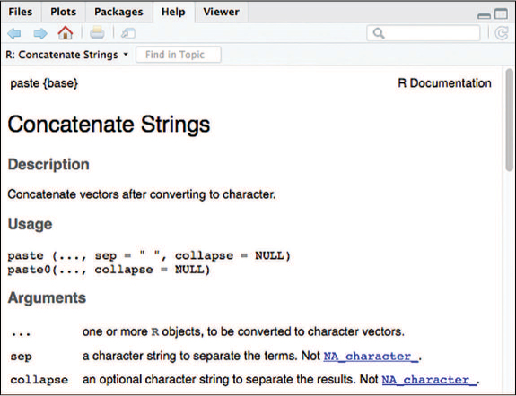
paste() function, as shown in RStudio.
Tip
In R’s documentation, functions that require a limited number of unnamed arguments will often refer to them as x. For example, the documentation for round() is listed as follows: round(x, digits = 0). The x just means “the data value to run this function on.”
Fun Fact
The mathematical operators (e.g., +) are actually functions in R that take two arguments (the operands). The familiar mathematical notation is just a shortcut.
# These two lines of code are the same:
x <- 2 + 3 # add 2 and 3
x <- '+'(2, 3) # add 2 and 3
6.3 Loading Functions
Although R comes with lots of built-in functions, you can always use more functions! Packages (also broadly, if inaccurately, referred to as libraries) are additional sets of R functions that are written and published by the R community. Because many R users encounter the same data management and analysis challenges, programmers are able to use these packages and thereby benefit from the work of others. (This is the amazing thing about the open source community—people solve problems and then make those solutions available to others.) Popular R packages exist for manipulating data (dplyr), making beautiful graphics (ggplot2), and implementing machine learning algorithms (randomForest).
R packages do not ship with the R software by default, but rather need to be downloaded (once) and then loaded into your interpreter’s environment (each time you wish to use them). While this may seem cumbersome, the R software would be huge and slow if you had to install and load all available packages to do anything with it.
Luckily, it is possible to install and load R packages from within R. The base R software provides install.packages() function for installing packages, and the library() function for loading them. The following example illustrates installing and loading the stringr package (which contains handy functions for working with character strings):
# Install the `stringr` package. Only needs to be done once per computer
install.packages("stringr")

# Load the package (make `stringr` functions available in this `R` session)
library("stringr") # quotes optional here, but best to include them
Caution
When you install a package, you may receive a warning message about the package being built under a previous version of R. In all likelihood, this shouldn’t cause a problem, but you should pay attention to the details of the messages and keep them in mind (especially if you start getting unexpected errors).
Errors installing packages are some of the trickiest to solve, since they depend on machine-specific configuration details. Read any error messages carefully to determine what the problem may be.
The install.packages() function downloads the necessary set of R code for a given package (which explains why you need to do it only once per machine), while the library() function loads those scripts into your current R session (you connect to the “library” where the package has been installed). If you’re curious where the library of packages is located on your computer, you can run the R function .libPaths() to see where the files are stored.
Caution
Loading a package sometimes overrides a function of the same name that is already in your environment. This may cause a warning to appear in your R terminal, but it does not necessarily mean you made a mistake. Make sure to read warning messages carefully and attempt to decipher their meaning. If the warning doesn’t refer to something that seems to be a problem (such as overriding existing functions you weren’t going to use), you can ignore it and move on.
After loading a package with the library() function, you have access to functions that were written as part of that package. For example, stringr provides a function str_count() that returns how many times a “substring” appears in a word (see the stringr documentation3 for a complete list of functions included in that package):
3https://cran.r-project.org/web/packages/stringr/stringr.pdf
# How many i's are in Mississippi?
str_count("Mississippi", "i") # 4
Because there are so many packages, many of them will provide functions with the same names. You thus might need to distinguish between the str_count() function from stringr and the str_count() function from somewhere else. You can do this by using the full package name of the function (called namespacing the function)—written as the package name, followed by a double colon (::), followed by the name of the function:
# Explicitly call the namespaced `str_count` function. Not very common.
stringr::str_count("Mississippi", "i") # 4

# Equivalently, call the function without namespacing
str_count("Mississippi", "i") # 4
Much of the work involved in programming for data science involves finding, understanding, and using these external packages (no need to reinvent the wheel!). A number of such packages will be discussed and introduced in this text, but you must also be willing to extrapolate what you learn (and research further examples) to new situations.
Tip
There are packages available to help you improve the style of your R code. The lintra package detects code that violates the tidyverse style guide, and the stylerb package applies suggested formatting to your code. After loading those packages, you can run lint("MY_FILENAME.R") and style_file("MY_FILENAME.R") (using the appropriate filename) to help ensure you have used good code style.
6.4 Writing Functions
Even more exciting than loading other people’s functions is writing your own. Anytime that you have a task that you may repeat throughout a script—or if you just want to organize your thinking—it’s good practice to write a function to perform that task. This will limit repetition and reduce the likelihood of errors, as well as make things easier to read and understand (and identify flaws in your analysis).
The best way to understand the syntax for defining a function is to look at an example:
# A function named `make_full_name` that takes two arguments
# and returns the "full name" made from them
make_full_name <- function(first_name, last_name) {
  # Function body: perform tasks in here
  full_name <- paste(first_name, last_name)

  # Functions will *return* the value of the last line
  full_name
}

# Call the `make_full_name()` function with the values "Alice" and "Kim"
my_name <- make_full_name("Alice", "Kim") # returns "Alice Kim" into `my_name`
Functions are in many ways like variables: they have a name to which you assign a value (using the same assignment operator: <-). One difference is that they are written using the function keyword to indicate that you are creating a function and not simply storing a value. Per the tidyverse style guide,4 functions should be written in snake_case and named using verbs—after all, they define something that the code will do. A function’s name should clearly suggest what it does (without becoming too long).
4tidyverse style Guide: http://style.tidyverse.org/functions.html
Remember
Although tidyverse functions are written in snake_case, many built-in R functions use a dot . to separate words—for example, install.packages() and is.numeric() (which determines whether a value is a number and not, for example, a character string).
A function includes several different parts:
Arguments: The value assigned to the function name uses the syntax
function(...)to indicate that you are creating a function (as opposed to a number or character string). The words put between the parentheses are names for variables that will contain the values passed in as arguments. For example, when you callmake_full_name("Alice", "Kim"), the value of the first argument ("Alice") will be assigned to the first variable (first_name), and the value of the second argument ("Kim") will be assigned to the second variable (last_name).Importantly, you can make the argument names anything you want (
name_first,given_name, and so on), just as long as you then use that variable name to refer to the argument inside the function body. Moreover, these argument variables are available only while inside the function. You can think of them as being “nicknames” for the values. The variablesfirst_name,last_name, andfull_nameexist only within this particular function; that is, they are accessible within the scope of the function.Body: The body of the function is a block of code that falls between curly braces
{}(a “block” is represented by curly braces surrounding code statements). The cleanest style is to put the opening{immediately after the arguments list, and the closing}on its own line.The function body specifies all the instructions (lines of code) that your function will perform. A function can contain as many lines of code as you want. You will usually want more than 1 line to make the effort of creating the function worthwhile, but if you have more than 20 lines, you might want to break it up into separate functions. You can use the argument variables in here, create new variables, call other functions, and so on. Basically, any code that you would write outside of a function can be written inside of one as well!
Return value: A function will return (output) whatever value is evaluated in the last statement (line) of that function. In the preceding example, the final
full_namestatement will be returned.It is also possible to explicitly state what value to return by using the
return()function, passing it the value that you wish your function to return:# A function to calculate the area of a rectangle calculate_rect_area <- function(width, height){ return(width * height) # return a specific result }
However, it is considered good style to use the
return()statement only when you wish to return a value before the final statement is executed (see Section 6.5). As such, you can place the value you wish to return as the last line of the function, and it will be returned:# A function to calculate the area of a rectangle calculate_rect_area <- function(width, height){ # Store a value in a variable, then return that value area <- width * height # calculate area area # return this value from the function } # A function to calculate the area of a rectangle calculate_rect_area <- function(width, height){ # Equivalently, return a value anonymously (without first storing it) width * height # return this value from the function }
You can call (execute) a function you defined the same way you call built-in functions. When you do so, R will take the arguments you pass in (e.g., "Alice" and "Kim") and assign them to the argument variables. It then executes each line of code in the function body one at a time. When it gets to the last line (or the return() call), it will end the function and return the last expression, which could be assigned to a different variable outside of the function.
Overall, writing functions is an effective way to group lines of code together, creating an abstraction for those statements. Instead of needing to think about doing four or five steps at once, you can just think about a single step: calling the function! This makes it easier to understand your code and the analysis you need to perform.
6.4.1 Debugging Functions
A central part of writing functions is fixing the (inevitable) errors that you introduce in the process. Identifying errors within the functions you write is more complex than resolving an issue with a single line of code because you will need to search across the entire function to find the source of the error! The best technique for honing in on and identifying the line of code with the error is to run each line of code one at a time. While it is possible to execute each line individually in RStudio (using cmd+enter), this process requires further work when functions require arguments.
For example, consider a function that calculates a person’s body mass index (BMI):
# Calculate body mass index (kg/m^2) given the input in pounds (lbs) and
# inches (inches)
calculate_bmi <- function(lbs, inches) {
  height_in_meters <- inches * 0.0254
  weight_in_kg <- lbs * 0.453592
  bmi <- weight_in_kg / height_in_meters ^ 2
  bmi
}

# Calculate the BMI of a person who is 180 pounds and 70 inches tall
calculate_bmi(180, 70)
Recall that when you execute a function, R evaluates each line of code, replacing the arguments of that function with the values you supply. When you execute the function (e.g., by calling calculate_bmi(180, 70)), you are essentially replacing the variable lbs with the value 180, and replacing the variable inches with the value 70 throughout the function.
But if you try to run each statement in the function one at a time, then the variables lbs and inches won’t have values (because you never actually called the function)! Thus a strategy for debugging functions is to assign sample values to your arguments, and then run through the function line by line. For example, you could do the following (either within the function, in another part of the script, or just in the console):
# Set sample values for the `lbs` and `inches` variables
lbs <- 180
inches <- 70
With those variables assigned, you can run each statement inside the function one at a time, checking the intermediate results to see where your code makes a mistake—and then you can fix that line and retest the function! Be sure to delete the temporary variables when you’re done.
Note that while this will identify syntax errors, it will not help you identify logical errors. For example, this strategy will not help if you use the incorrect conversion between inches and meters, or pass the arguments to your function in the incorrect order. For example, calculate_bmi(70, 180) won’t return an error, but it will return a very different BMI than calculate_bmi(180, 70).
Remember
When you pass arguments to functions, order matters! Be sure that you are passing in values in the order expected by the function.
6.5 Using Conditional Statements
Functions are a way to organize and control the flow of execution of your code (e.g., which lines of code get run in which order). In R, as in other languages, you can also control program flow by specifying different instructions that can be run based on a different set of conditions. Conditional statements allow you to specify different blocks of code to run when given different contexts, which is often valuable within functions.
In an abstract sense, a conditional statement is saying:
IF something is true
  do some lines of code
OTHERWISE
  do some other lines of code
In R, you write these conditional statements using the keywords if and else and the following syntax:
# A generic conditional statement
if (condition) {
  # lines of code to run if `condition` is TRUE
} else {
  # lines of code to run if `condition` is FALSE
}
Note that the else needs to be on the same line as the closing curly brace (}) of the if block. It is also possible to omit the else and its block, in case you don’t want to do anything when the condition isn’t met.
The condition can be any variable or expression that resolves to a logical value (TRUE or FALSE). Thus both of the following conditional statements are valid:
# Evaluate conditional statements based on the temperature of porridge

# Set an initial temperature value for the porridge
porridge_temp <- 125 # in degrees F

# If the porridge temperature exceeds a given threshold, enter the code block
if (porridge_temp > 120) { # expression is true
  print("This porridge is too hot!") # will be executed
}

# Alternatively, you can store a condition (as a TRUE/FALSE value)
# in a variable
too_cold <- porridge_temp < 70 # a logical value

# If the condition `too_cold` is TRUE, enter the code block
if (too_cold) { # expression is false
  print("This porridge is too cold!") # will not be executed
}
You can further extend the set of conditions evaluated using an else if statement (e.g., an if immediately after an else). For example:
# Function to determine if you should eat porridge
test_food_temp <- function(temp) {
  if (temp > 120) {
    status <- "This porridge is too hot!"
  } else if (temp < 70) {
    status <- "This porridge is too cold!"
  } else {
    status <- "This porridge is just right!"
  }
  status # return the status
}

# Use the function on different temperatures
test_food_temp(150) # "This porridge is too hot!"
test_food_temp(60)  # "This porridge is too cold!"
test_food_temp(119) # "This porridge is just right!"
Note that a set of conditional statements causes the code to branch—that is, only one block of the code will be executed. As such, you may want to have one block return a specific value from a function, while the other block might keep going (or return something else). This is when you would want to use the return() function:
# Function to add a title to someone's name
add_title <- function(full_name, title) {
  # If the name begins with the title, just return the name
  if (startsWith(full_name, title)) {
    return(full_name) # no need to prepend the title
  }

  name_with_title <- paste(title, full_name) # prepend the title
  name_with_title # last argument gets returned
}
Note that this example didn’t use an explicit else clause, but rather just let the function “keep going” when the if condition wasn’t met. While both approaches would be valid (achieve the same desired result), it’s better code design to avoid `else` statements when possible and to instead view the if conditional as just handling a “special case.”
Overall, conditionals and functions are ways to organize the flow of code in your program: to explicitly tell the R interpreter in which order lines of code should be executed. These structures become particularly useful as programs get large, or when you need to combine code from multiple script files. For practice using and writing functions, see the set of accompanying book exercises.5
5Function exercises: https://github.com/programming-for-data-science/chapter-06-exercises