18
Dynamic Reports with R Markdown
The insights you discover through your analysis are only valuable if you can share them with others. To do this, it’s important to have a simple, repeatable process for combining the set of charts, tables, and statistics you generate into an easily presentable format.
This chapter introduces R Markdown1 as a tool for compiling and sharing your results. R Markdown is a development framework that supports using R to dynamically create documents, such as websites (.html files), reports (.pdf files), and even slideshows (using ioslides or slidy).
1R Markdown: https://rmarkdown.rstudio.com
As you may have guessed, R Markdown does this by providing the ability to blend Markdown syntax and R code so that, when compiled and executed, the results from your code will be automatically injected into a formatted document. The ability to automatically generate reports and documents from a computer script eliminates the need to manually update the results of a data analysis project, enabling you to more effectively share the information that you’ve produced from your data. In this chapter, you will learn the fundamentals of the R Markdown package so that you can create well-formatted documents that combine analysis and reporting.
Fun Fact
This book was written using R Markdown!
18.1 Setting Up a Report
R Markdown documents are created from a combination of two packages: rmarkdown (which processes the markdown and generates the output) and knitr2 (which runs R code and produces Markdown-like output). These packages are produced by and already included in RStudio, which provides direct support for creating and viewing R Markdown documents.
2knitr package: https://yihui.name/knitr/
18.1.1 Creating .Rmd Files
The easiest way to create a new R Markdown document in RStudio is to use the File > New File > R Markdown menu option (see Figure 18.1), which opens a document creation wizard.

File > New File > R Markdown).
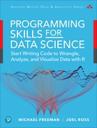
RStudio will then prompt you to provide some additional details about what kind of R Markdown document you want to create (shown in Figure 18.2). In particular, you will need to choose a default document type and output format. You can also provide a title and author information that will be included in the document. This chapter focuses on creating HTML documents (websites, the default format); other formats require the installation of additional software.
Once you’ve chosen your desired document type and output format, RStudio will open up a new script file for you. You should save this file with the extension .Rmd (for “R Markdown”), which tells the computer and RStudio that the document contains Markdown content with embedded R code. If you use a different extension, RStudio won’t know how to interpret the code and render the output!
The wizard-generated file contains some example code demonstrating how to write an R Markdown document. Understanding the basic structure of this file will enable you to insert your own content into this structure.
A .Rmd file has three major types of content: the header, the Markdown content, and R code chunks.
The header is found at the top of the file, and includes text with the following format:
---
title: "EXAMPLE_TITLE"
author: "YOUR_NAME"
date: "2/01/2018"
output: html_document
---
This header is written in YAML3 format, which is yet another way of formatting structured data, similar to CSV or JSON. In fact, YAML is a superset of JSON and can represent the same data structures, just using indentation and dashes instead of braces and commas.
3YAML: http://yaml.org
The header contains meta-data, or information about the file and how it should be processed and rendered. For example, the
title,author, anddatewill be automatically included and displayed at the top of your generated document. You can include additional information and configuration options as well, such as whether there should be a table of contents. See the R Markdown documentation4 for further details.4R Markdown HTML Documents: http://rmarkdown.rstudio.com/html_document_format.html
Everything below the header is the content that will be included in your report, and is primarily made up of Markdown content. This is normal Markdown text like that described in Chapter 4. For example, you could include the following markdown code in your
.Rmdfile:## Second Level Header This is just plain markdown that can contain **bold** or _italics_.R Markdown also provides the ability to render code content inline with the Markdown content, as described later in this chapter.
R code chunks can be included in the middle of the regular Markdown content. These segments (chunks) of
Rcode look like normal code block elements (using three backticks```), but with an extra{r}immediately after the opening set of backticks. Inside these code chunks you include regularRcode, which will be evaluated and then rendered into the document. Section 18.2 provides more details about the format and process used by these chunks.```{r} # R code chunk in an R Markdown file some_variable <- 100 ```
Combining these content types (header, markdown, and code chunks), you will be able to reproducibly create documents to share your insights.
18.1.2 Knitting Documents
RStudio provides a direct interface to compile your .Rmd source code into an actual document (a process called knitting, performed by the knitr package). To do so, click the Knit button at the top of the script panel, shown in Figure 18.3. This button will compile the code and generate the document (into the same directory as your saved .Rmd file), as well as open up a preview window in RStudio.

While it is straightforward to generate such documents, the knitting process can make it hard to debug errors in your R code (whether syntax or logical), in part because the output may or may not show up in the document! We suggest that you write complex R code in another script and then use the source() function to insert that script into your .Rmd file and use calculated variables in your output (see Chapter 14 for details and examples of the source() function). This makes it possible to test your data processing work outside of the knitted document. It also separates the concerns of the data and its representation—which is good programming practice.
Nevertheless, you should be sure to knit your document frequently, paying close attention to any errors that appear in the console.
Tip
If you’re having trouble finding your error, a good strategy is to systematically remove (“comment out”) segments of your code and attempt to re-knit the document. This will help you identify the problematic syntax.
18.2 Integrating Markdown and R Code
What makes R Markdown distinct from simple Markdown code is the ability to actually execute your R code and include the output directly in the document. R code can be executed and included in the document in blocks of code, or even inline with other content!
18.2.1 R Code Chunks
Code that is to be executed (rather than just displayed as formatted text) is called a code chunk. To specify a code chunk, you need to include {r} immediately after the backticks that start the code block (the ```). You can type this out yourself, or use the keyboard shortcut (cmd+alt+i) to create one. For example:
Write normal **markdown** out here, then create a code block:

```{r}
# Execute R code in here
course_number <- 201
```

Back to writing _markdown_ out here.
By default, the code chunk will execute the R code listed, and then render both the code that was executed and the result of the last statement into the Markdown—similar to what would be returned by a function. Indeed, you can think of code chunks as functions that calculate and return a value that will be included in the rendered report. If your code chunk doesn’t return a particular expression (e.g., the last line is just an assignment), then no returned output will be rendered, although R Markdown will still render the code that was executed.
It is also possible to specify additional configuration options by including a comma-separated list of named arguments (as you’ve done with lists and functions) inside the curly braces following the r:
```{r options_example, echo = FALSE, message = TRUE)
# A code chunk named "options_example", with argument `echo` assigned FALSE
# and argument `message` assigned TRUE

# Would execute R code in here
```
The first “argument” (options_example) is a “name” or label for the chunk; it is followed by named arguments (written in option = VALUE format) for the options. While including chunk names is technically optional, this practice will help you create well-documented code and reference results in the text. It will also help in the debugging process, as it will allow RStudio to produce more detailed error messages.
There are many options5 you can use when creating code chunks. Some of the most useful ones have to do with how the executed code is output in the document:
5knitr Chunk options and package options: https://yihui.name/knitr/options/
echoindicates whether you want the R code itself to be displayed in the document (i.e., if you want readers to be able to see your work and reproduce your calculations and analysis). The value is eitherTRUE(do display; the default) orFALSE(do not display).messageindicates whether you want any messages generated by the code to be displayed. This includes print statements! The value is eitherTRUE(do display; the default) orFALSE(do not display).includeindicates if any results of the code should be output in the report. Note that any code in this chunk will still be executed—it just won’t be included in the output. It is extremely common and best practice to have a “setup” code chunk at the beginning of your report that has theinclude = FALSEoption and is used to do initial processing work—such aslibrary()packages,source()analysis code, or perform some other data wrangling. The R Markdown reports produced by RStudio’s wizard include a code chunk like this.
If you want to show your R code but not evaluate it, you can use a standard Markdown code block that indicates the r language (```r instead of ```{r}), or set the eval option to FALSE.
18.2.2 Inline Code
In addition to creating distinct code blocks, you will commonly want to execute R code inline with the rest of your text. This empowers you to reference a variable defined in a code chunk in a section of Markdown—injecting the value stored in a variable into the text you have written. Using this technique, you can include a specific result inside a paragraph of text; if the computation changes, re-knitting your document will update the values inside the text without any further work needed.
Recall that a single backtick (`) is the Markdown syntax for making text display as code. You can make R Markdown evaluate—rather than display—inline code by adding the letter r and a space immediately after the first backtick. For example:
To calculate 3 + 4 inside some text, you can use `r 3 + 4` right in the _middle_.
When you knit this text, `r 3 + 4` would be replaced with the number 7 (what 3 + 4 evaluates to).
You can also reference values computed in any code chunks that precede the inline code. For example, `r SOME_VARIABLE` would include the value of SOME_VARIABLE inline with the paragraph. In fact, it is best practice to do your calculations in a code block (with the echo = FALSE option), save the result in a variable, and then inline that variable to display it.
Tip
To quickly access the R Markdown Cheatsheet and Reference, use the RStudio menu: Help > Cheatsheets.
18.3 Rendering Data and Visualizations in Reports
R Markdown’s code chunks let you perform data analysis directly in your document, but you will often want to include more complex data output than just the resulting numbers. This section discusses a few tips for specifying dynamic, complex output to render using R Markdown.
18.3.1 Rendering Strings
If you experiment with knitting R Markdown, you will quickly notice that using print() will generate content that looks like a printed vector (e.g., what you see in the console in RStudio). For example:
```{r raw_print_example, echo = FALSE}
print("Hello world")
```
will produce:
## [1] "Hello world"
For this reason, you usually want to have the code block generate a string that you save in a variable, which you can then display with an inline expression (e.g., on its own line):
```{r stored_print_example, echo = FALSE}
msg <- "**Hello world**"
```

Below is the message to see:

`r msg`
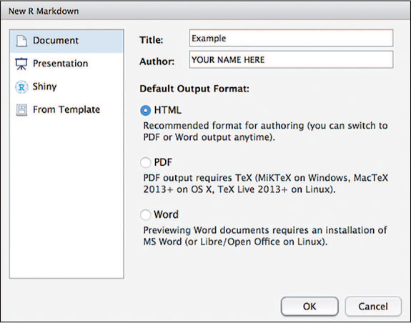
When knit, this code produces the text shown in Figure 18.4. Note that the Markdown syntax included in the variable is rendered as well: `r msg` is replaced by the value of the expression just as if you had typed that Markdown in directly. This allows you to even include dynamic styling if you construct a “Markdown string” (i.e., containing Markdown syntax) from your data.
.html file that is created by knitting an R Markdown document containing a chunk that stores a message in a variable and an inline expression of that message.Alternatively, you can give your chunk a results option6 with a value "asis", which will cause the output to be rendered directly into the Markdown. When combined with the base R function cat() (which concatenates content without specifying additional information such as vector position), you can make a code chunk effectively render a specific string:
6knitr text result options: https://yihui.name/knitr/options/#text-results
```{r asis_example, results = "asis", echo = FALSE}
cat("**Hello world**")
```
18.3.2 Rendering Markdown Lists
Because output strings render any Markdown they contain, it’s possible to construct these Markdown strings so that they contain more complex structures such as unordered lists. To do this, you specify the string to include the - symbols used to indicate a Markdown list (with each item in the list separated by a line break or a
character):
```{r list_example, echo = FALSE}
markdown_list <- "
- Lions
- Tigers
- Bears
- Oh mys
"
```

`r markdown_list`
This code outputs a list that looks like this:
Lions
Tigers
Bears
Oh mys
When this approach is combined with the vectorized paste() function and its collapse argument, it becomes possible to convert vectors into Markdown lists that can be rendered:
```{r pasted_list_example, echo = FALSE}
# Create a vector of animals
animals <- c("Lions", "Tigers", "Bears", "Oh mys")

# Paste `-` in front of each animal and join the items together with
# newlines between
markdown_list <- paste("-", animals, collapse = "n")
```

`r markdown_list`
Of course, the contents of the vector (e.g., the text "Lions") could include additional Markdown syntax to make it bold, italic, or hyperlinked text.
Tip
Creating a “helper function” to help with formatting your output is a great approach. For some other work in this area, see the pandera package.
18.3.3 Rendering Tables
Because data frames are so central to programming with R, R Markdown includes capabilities that enable you to render data frames as Markdown tables via the knitr package’s kable() function. This function takes as an argument the data frame you wish to render, and it will automatically convert that value into a string of text representing a Markdown table:
```{r kable_example, echo = FALSE}
library("knitr") # make sure you load the package (once per document)

# Make a data frame
letters <- c("a", "b", "c", "d")
numbers <- 1:4
df <- data.frame(letters = letters, numbers = numbers)

# "Return" the table to render it
kable(df)
```
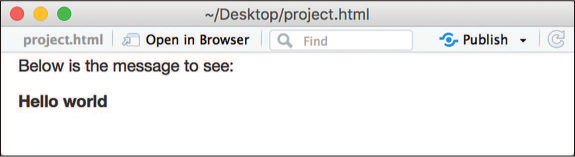
Figure 18.5 compares the rendered R Markdown results with and without the kable() function. The kable() function supports a number of other arguments that can be used to customize how it outputs a table; see the documentation for details. Again, if the values in the data frame are strings that contain Markdown syntax (e.g., bold, italics, or hyperlinks), they will be rendered as such in the table!
kable() function.
Going Further
So while you may need to do a little bit of work to manually generate the Markdown syntax, R Markdown makes it is possible to dynamically produce complex documents based on dynamic data sources.
18.3.4 Rendering Plots
You can also include visualizations created by R in your rendered reports! To do so, you have the code chunk “return” the plot you wish to render:
```{r plot_example, echo = FALSE}
library("ggplot2") # make sure you load the package (once per document)

# Plot of college education vs. poverty rates in the Midwest
ggplot(data = midwest) +
  geom_point(
    mapping = aes(x = percollege, y = percadultpoverty, color = state)
  ) +
  scale_color_brewer(palette = "Set3")
```
When knit, the document generated that includes this code would include the ggplot2 chart. Moreover, RStudio allows you to preview each code chunk before knitting—just click the green play button icon above each chunk, as shown in Figure 18.6. While this can help you debug individual chunks, it may be tedious to do in longer scripts, especially if variables in one code chunk rely on an earlier chunk.

knitr is displayed when you click the green play button icon (very helpful for debugging .Rmd files!).
It is best practice to do any data wrangling necessary to prepare the data for your plot in a separate .R file, which you can then source() into the R Markdown (in an initial setup code chunk with the include = FALSE option). See Section 18.5 for an example of this organization.
18.4 Sharing Reports as Websites
The default output format for new R Markdown scripts created with RStudio is HTML (with the content saved in a .html file). HTML stands for HyperText Markup Language and, like the Markdown language, is a syntax for describing the structure and formatting of content (though HTML is far more extensive and detailed). In particular, HTML is a markup language that can be automatically rendered by web browsers, so it is the language used to create webpages. In fact, you can open up .html files generated by RStudio in any web browser to see the content. Additionally, this means that the .html files you create with R Markdown can be put online as webpages for others to view!
As it turns out, you can use GitHub not only to host versions of your code repository, but also to serve (display) .html files—including ones generated from R Markdown. Github will host webpages on a publicly accessible web server that can “serve” the page to anyone who requests it (at a particular URL on the github.io domain). This feature is known as GitHub Pages.7
7What Is GitHub Pages: https://help.github.com/articles/what-is-github-pages/
Using GitHub Pages involves a few steps. First, you need to knit your document into a .html file with the name index.html—this is the traditional name for a website’s homepage (and the file that will be served at a particular URL by default). You will need to have pushed this file to a GitHub repository; the index.html file will need to be in the root folder of the repo.
Next, you need to configure that GitHub repository to enable GitHub Pages. On the web portal page for your repo, click on the “Settings” tab, and scroll down to the section labeled “GitHub Pages.” From there, you need to specify the “Source” of the .html file that Github Pages should serve. Select the “master branch” option to enable GitHub Pages and have it serve the “master” version of your index.html file (see Figure 18.7).

master branch to host your compiled index.html file as a website!Going Further
Once you’ve enabled GitHub Pages, you will be able to view your hosted webpage at the URL:
# The URL for a website hosted with GitHub Pages
https://GITHUB_USERNAME.github.io/REPO_NAME
Replace GITHUB_USERNAME with the username of the account hosting the repo, and REPO_NAME with your repository name. Thus, if you pushed your code to the mkfreeman/report repo on GitHub (stored online at https://github.com/mkfreeman/report), the webpage would be available at https://mkfreeman.github.io/report. See the official documentation8 for more details and options.
8Documentation for GitHub Pages: https://help.github.com/articles/user-organization-and-project-pages/
18.5 R Markdown in Action: Reporting on Life Expectancy
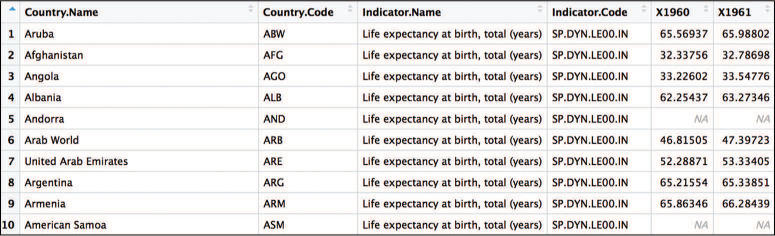
To demonstrate the power of using R Markdown as a tool to generate dynamic reports, this section walks through authoring a report about the life expectancy in each country from 1960 to 2015. The data for the example can be downloaded from the World Bank.9 The complete code for this analysis is also available online in the book code repository.10 A subset of the data is shown in Figure 18.8.
9World Bank: life expectancy at birth data: https://data.worldbank.org/indicator/SP.DYN.LE00.IN
10R Markdown in Action: https://github.com/programming-for-data-science/in-action/tree/master/r-markdown
To keep the code organized, the report will be written in two separate files:
analysis.R, which will contain the analysis and save important values in variablesindex.Rmd, which willsource()theanalysis.Rscript, and generate the report (the file is named so that it can be hosted on GitHub Pages when rendered)
The analysis.R file will need to complete the following tasks:
Load the data.
Compute metrics of interest.
Generate data visualizations to display.
As each step is completed in this file, key reporting values and charts are saved to variables so that they can be referenced in the index.Rmd file.
To reference these variables, you load the analysis.R script (with source()) in a “setup” block of the index.Rmd file, enabling its data to be referenced within the Markdown. The include = FALSE code chunk option means that the block will be evaluated, but not rendered in the document.
```{r setup, include = FALSE}
# Load results from the analysis
# Errors and messages will not be printed because `include` is set to FALSE
source("analysis.R")
```
Remember
All “algorithmic” work should be done in the separate analysis.R file, allowing you to more easily debug and iterate your analysis. Since visualizations are part of the “presented” information, they could instead be generated directly in the R Markdown, though the data to be visualized should be preprocessed in the analysis.R file.
To compute the metrics of interest in your analysis.R file, you can use dplyr functions to ask questions of the data set. For example:
# Load the data, skipping unnecessary rows
life_exp <- read.csv(
  "data/API_SP.DYN.LE00.IN_DS2_en_csv_v2.csv",
  skip = 4,
  stringsAsFactors = FALSE
)

# Which country had the longest life expectancy in 2015?
longest_le <- life_exp %>%
  filter(X2015 == max(X2015, na.rm = T)) %>%
  select(Country.Name, X2015) %>%
  mutate(expectancy = round(X2015, 1)) # rename and format column
In this example, the data frame longest_le stores an answer to the question Which country had the longest life expectancy in 2015? This data frame could be included directly as content of the index.Rmd file. You will be able to reference values from this data frame inline to ensure the report contains the most up-to-date information, even if the data in your analysis changes:
The data revealed that the country with the longest life expectancy is
`r longest_le$Country.Name`, with a life expectancy of
`r longest_le$expectancy`.
When rendered, this code snippet would replace `r longest_le$Country.Name` with the value of that variable. Similarly, if you want to show a table as part of your report, you can construct a data frame with the desired information in your analysis.R script, and render it in your index.Rmd file using the kable() function:
# What are the 10 countries that experienced the greatest gain in
# life expectancy?
top_10_gain <- life_exp %>%
  mutate(gain = X2015 - X1960) %>%
  top_n(10, wt = gain) %>% # a handy dplyr function!
  arrange(-gain) %>%
  mutate(gain_str = paste(format(round(gain, 1), nsmall = 1),"years")) %>%
  select(Country.Name, gain_formatted)
Once you have stored the desired information in the top_10_gain data frame in your analysis.R script, you can display that information in your index.Rmd file using the following syntax:
```{r top_10_gain, echo = FALSE}
# Show the top 10 table (specifying the column names to display)
kable(top_10_gain, col.names = c("Country", "Change in Life Expectancy"))
```
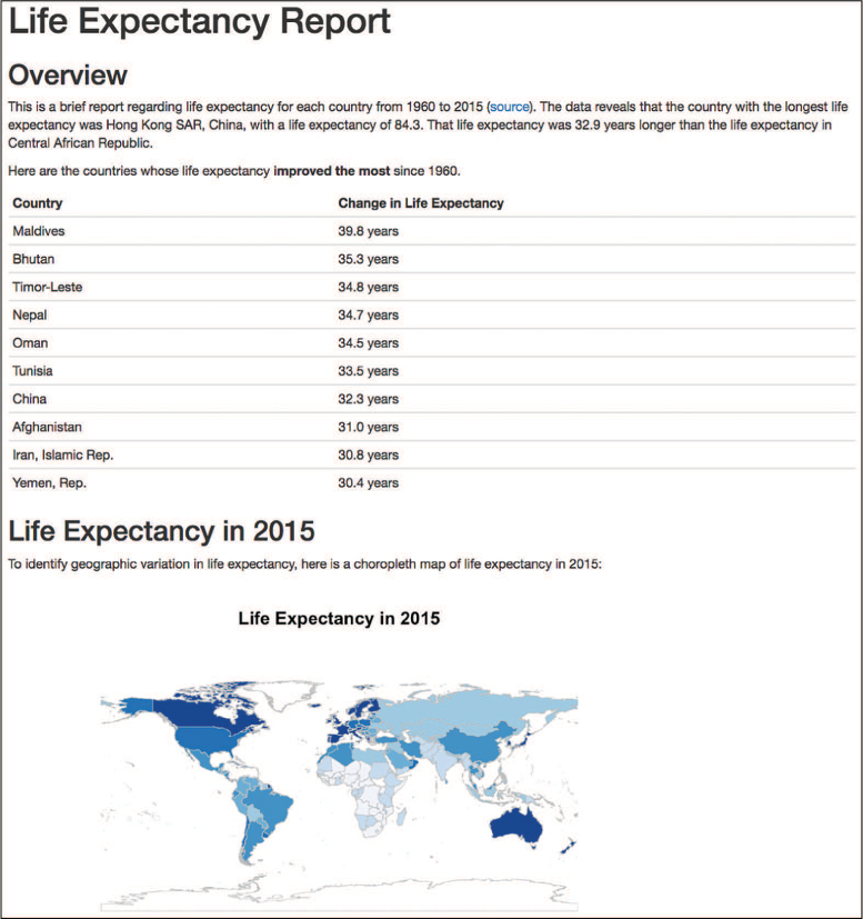
Figure 18.9 shows the entire report; the complete analysis and R Markdown code to generate this report follows. Note that the report uses a package called rworldmap to quickly generate a simple, static world map (as an alternative to mapping with ggplot2).
# analysis.R script

# Load required libraries
library(dplyr)
library(rworldmap) # for easy mapping
library(RColorBrewer) # for selecting a color palette

# Load the data, skipping unnecessary rows
life_exp <- read.csv(
  "data/API_SP.DYN.LE00.IN_DS2_en_csv_v2.csv",
  skip = 4,
  stringsAsFactors = FALSE
)

# Notice that R puts the letter "X" in front of each year column,
# as column names can't begin with numbers

# Which country had the longest life expectancy in 2015?
longest_le <- life_exp %>%
  filter(X2015 == max(X2015, na.rm = T)) %>%
  select(Country.Name, X2015) %>%
  mutate(expectancy = round(X2015, 1)) # rename and format column

# Which country had the shortest life expectancy in 2015?
shortest_le <- life_exp %>%
  filter(X2015 == min(X2015, na.rm = T)) %>%
  select(Country.Name, X2015) %>%
  mutate(expectancy = round(X2015, 1)) # rename and format column

# Calculate range in life expectancies
le_difference <- longest_le$expectancy - shortest_le$expectancy

# What 10 countries experienced the greatest gain in life expectancy?
top_10_gain <- life_exp %>%
  mutate(gain = X2015 - X1960) %>%
  top_n(10, wt = gain) %>% # a handy dplyr function!
  arrange(-gain) %>%
  mutate(gain_str = paste(format(round(gain, 1), nsmall = 1), "years")) %>%
  select(Country.Name, gain_str)
# Join this data frame to a shapefile that describes how to draw each country
# The `rworldmap` package provides a helpful function for doing this
mapped_data <- joinCountryData2Map(
  life_exp,
  joinCode = "ISO3",
  nameJoinColumn = "Country.Code",
  mapResolution = "high"
)
The following index.Rmd file renders the report using the preceding analysis.R script:
---
title: "Life Expectancy Report"
output: html_document
---

```{r setup, include = FALSE}
# Load results from the analysis
# errors and messages will not be printed given the `include = FALSE` option
source("analysis.R")

# Also load additional libraries that may be needed for output
library("knitr")
```

## Overview
This is a brief report regarding life expectancy for each country from
1960 to 2015 ([source](https://data.worldbank.org/indicator/SP.DYN.LE00.IN)).
The data reveals that the country with the longest life expectancy was
`r longest_le$Country.Name`, with a life expectancy of
`r longest_le$expectancy`. That life expectancy was `r le_difference`
years longer than the life expectancy in `r shortest_le$Country.Name`.

Here are the countries whose life expectancy **improved the most** since 1960.

```{r top_10_gain, echo = FALSE}
# Show the top 10 table (specifying the column names to display)
kable(top_10_gain, col.names = c("Country", "Change in Life Expectancy"))
```

## Life Expectancy in 2015
To identify geographic variations in life expectancy,
here is a choropleth map of life expectancy in 2015:

```{r le_map, echo = FALSE}
# Create and render a world map using the `rworldmap` package
mapCountryData(
  mapped_data, # indicate the data to map
  mapTitle = "Life Expectancy in 2015",
  nameColumnToPlot = "X2015",
  addLegend = F, # exclude the legend
  colourPalette = brewer.pal(7, "Blues") # set the color palette
)
```
For practice creating reports with R Markdown, see the set of accompanying book exercises.11
11R Markdown exercises: https://github.com/programming-for-data-science/chapter-18-exercises