7
Vectors
As you move from practicing R basics to interacting with data, you will need to understand how that data is stored, and to carefully consider the appropriate structure for the organization, analysis, and visualization of your data. This chapter covers the foundational concepts for working with vectors in R. Vectors are the fundamental data type in R, so understanding these concepts is key to effectively programming in the language. This chapter discusses how R stores information in vectors, the way in which operations are executed in vectorized form, and how to extract data from vectors.
7.1 What Is a Vector?
Vectors are one-dimensional collections of values that are all stored in a single variable. For example, you can make a vector people that contains the character strings “Sarah”, “Amit”, and “Zhang”. Alternatively, you could make a vector one_to_seventy that stores the numbers from 1 to 70. Each value in a vector is referred to as an element of that vector; thus the people vector would have three elements: "Sarah", "Amit", and "Zhang".
Remember
All the elements in a vector need to have the same type (e.g., numeric, character, logical). You can’t have a vector whose elements include both numbers and character strings.
7.1.1 Creating Vectors
The easiest and most common syntax for creating vectors is to use the built-in c() function, which is used to combine values into a vector. The c() function takes in any number of arguments of the same type (separated by commas as usual), and returns a vector that contains those elements:
# Use the `c()` function to create a vector of character values
people <- c("Sarah", "Amit", "Zhang")
print(people)
# [1] "Sarah" "Amit" "Zhang"
# Use the `c()` function to create a vector of numeric values
numbers <- c(1, 2, 3, 4, 5)
print(numbers)
# [1] 1 2 3 4 5
When you print out a variable in R, the interpreter prints out a [1] before the value you have stored in your variable. This is R telling you that it is printing from the first element in your vector (more on element indexing later in this chapter). When R prints a vector, it prints the elements separated with spaces (technically tabs), not commas.
You can use the length() function to determine how many elements are in a vector:
# Create and measure the length of a vector of character elements
people <- c("Sarah", "Amit", "Zhang")
people_length <- length(people)
print(people_length)
# [1] 3

# Create and measure the length of a vector of numeric elements
numbers <- c(1, 2, 3, 4, 5)
print(length(numbers))
# [1] 5
Other functions can also help with creating vectors. For example, the seq() function mentioned in Chapter 6 takes two arguments and produces a vector of the integers between them. An optional third argument specifies how many numbers to skip in each step:
# Use the `seq()` function to create a vector of numbers 1 through 70
# (inclusive)
one_to_seventy <- seq(1, 70)
print(one_to_seventy)
# [1] 1 2 3 4 5 .....

# Make vector of numbers 1 through 10, counting by 2
odds <- seq(1, 10, 2)
print(odds)
# [1] 1 3 5 7 9
As a shorthand, you can produce a sequence with the colon operator (a:b), which returns a vector from a to b with the element values being incremented by 1:
# Use the colon operator (:) as a shortcut for the `seq()` function
one_to_seventy <- 1:70
When you print out one_to_seventy (as in Figure 7.1), in addition to the leading [1] that you’ve seen in all printed results, there are bracketed numbers at the start of each line. These bracketed numbers tell you the starting position (index) of elements printed on that line. Thus the [1] means that the printed line shows elements starting at element number 1, a [28] means that the printed line shows elements starting at element number 28, and so on. This information is intended to help make the output more readable, so you know where in the vector you are when looking at a printed line of elements.

seq() function and printing the results in the RStudio terminal.
7.2 Vectorized Operations
When performing operations (such as mathematical operations +, -, and so on) on vectors, the operation is applied to vector elements element-wise. This means that each element from the first vector operand is modified by the element in the same corresponding position in the second vector operand. This will produce the value at the corresponding position of the resulting vector. In other words, if you want to add two vectors, then the value of the first element in the result will be the sum of the first elements in each vector, the second element in the result will be the sum of the second elements in each vector, and so on.
Figure 7.2 demonstrates the element-wise nature of the vectorized operations shown in the following code:
# Create two vectors to combine
v1 <- c(3, 1, 4, 1, 5)
v2 <- c(1, 6, 1, 8, 0)

# Create arithmetic combinations of the vectors
v1 + v2 # returns 4 7 5 9 5
v1 - v2 # returns 2 -5 3 -7 5
v1 * v2 # returns 3 6 4 8 0
v1 / v2 # returns 3 0.167 4 0.125 Inf

# Add a vector to itself (why not?)
v3 <- v2 + v2 # returns 2 12 2 16 0

# Perform more advanced arithmetic!
v4 <- (v1 + v2) / (v1 + v1) # returns 0.67 3.5 0.625 4.5 0.5

v3) is the sum of the first element in the first vector (v1) and the first element in the second vector (v2).
Vectors support any operators that apply to their “type” (i.e., numeric or character). While you can’t apply mathematical operators (namely, +) to combine vectors of character strings, you can use functions like paste() to concatenate the elements of two vectors, as described in Section 7.2.3.
7.2.1 Recycling
Recycling refers to what R does in cases when there are an unequal number of elements in two operand vectors. If R is tasked with performing a vectorized operation with two vectors of unequal length, it will reuse (recycle) elements from the shorter vector. For example:
# Create vectors to combine
v1 <- c(1, 3, 5, 1, 5)
v2 <- c(1, 2)

# Add vectors
v3 <- v1 + v2 # returns 2 5 6 3 6
In this example, R first combined the elements in the first position of each vector (1 + 1 = 2). Then, it combined elements from the second position (3 + 2 = 5). When it got to the third element (which was present only in v1), it went back to the beginning of v2 to select a value, yielding 5 + 1 = 6. This recycling is illustrated in Figure 7.3.
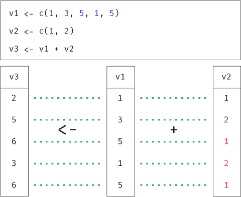
v2), the values will be repeated (recycled) to match the length of the longer vector. Recycled values are in red.
Remember
Recycling will occur no matter whether the longer vector is the first or the second operand. In either case, R will provide a warning message if the length of the longer vector is not a multiple of the shorter (so that there would be elements “left over” from recycling). This warning doesn’t necessarily mean you did something wrong, but you should pay attention to it because it may be indicative of an error (i.e., you thought the vectors were of the same length, but made a mistake somewhere).
7.2.2 Most Everything Is a Vector!
What happens if you try to add a vector and a “regular” single value (a scalar)?
# Add a single value to a vector of values
v1 <- 1:5 # create vector of numbers 1 to 5
result <- v1 + 4 # add scalar to vector
print(result)
# [1] 5 6 7 8 9
As you can see (and probably expected), the operation added 4 to every element in the vector.
This sensible behavior occurs because R stores all character, numeric, and boolean values as vectors. Even when you thought you were creating a single value (a scalar), you were actually creating a vector with a single element (length 1). When you create a variable storing the number 7 (e.g., with x <- 7), R creates a vector of length 1 with the number 7 as that single element.
# Confirm that basic types are stored in vectors
is.vector(18) # TRUE
is.vector("hello") # TRUE
is.vector(TRUE) # TRUE
This is why R prints the [1] in front of all results: it’s telling you that it’s showing a vector (which happens to have one element) starting at element number 1.
# Create a vector of length 1 in a variable `x`
x <- 7 # equivalent to `x <- c(7)`

# Print out `x`: R displays the vector index (1) in the console
print(x)
# [1] 7
This behavior explains why you can’t use the length() function to get the length of a character string; it just returns the length of the vector containing that string (which is 1). Instead, you would use the nchar() function to get the number of characters in a character string.
Thus when you add a “scalar” such as 4 to a vector, what you’re really doing is adding a vector with a single element 4. As such, the same recycling principle applies, so that the single element is recycled and applied to each element of the first operand.
7.2.3 Vectorized Functions
Because all basic data types are stored as vectors, almost every function you’ve encountered so far in this book can be applied to vectors, not just to single values. These vectorized functions are both more idiomatic and efficient than non-vector approaches. You will find that functions work the same way for vectors as they do for single values, because single values are just instances of vectors!
This means that you can use nearly any function on a vector, and it will act in the same vectorized, element-wise manner: the function will result in a new vector where the function’s transformation has been applied to each individual element in order.
For example, consider the round() function described in Chapter 6. This function rounds the given argument to the nearest whole number (or number of decimal places if specified).
# Round the number 1.67 to 1 decimal place
round(1.67, 1) # returns 1.7
But recall that the 1.67 in the preceding example is actually a vector of length 1. If you instead pass a vector containing multiple values as an argument, the function will perform the same rounding on each element in the vector.
# Create a vector of numbers
nums <- c(3.98, 8, 10.8, 3.27, 5.21)

# Perform the vectorized operation
rounded_nums <- round(nums, 1)

# Print the results (each element is rounded)
print(rounded_nums)
# [1]  4.0  8.0  10.8  3.3  5.2
Vectorized operations such as these are also possible with character data. For example, the nchar() function, which returns the number of characters in a string, can be used equivalently for a vector of length 1 or a vector with many elements inside of it:
# Create a character variable `introduction`, then count the number
# of characters
introduction <- "Hello"
nchar(introduction) # returns 5

# Create a vector of `introductions`, then count the characters in
# each element
introductions <- c("Hi", "Hello", "Howdy")
nchar(introductions) # returns 2  5  5
Remember
When you use a function on a vector, you’re using that function on each item in the vector!
You can even use vectorized functions in which each argument is a vector. For example, the following code uses the paste() function to paste together elements in two different vectors. Just as the plus operator (+) performed element-wise addition, other vectorized functions such as paste() are also implemented element-wise:
# Create a vector of two colors
colors <- c("Green", "Blue")

# Create a vector of two locations
locations <- c("sky", "grass")

# Use the vectorized paste() operation to paste together the vectors above
band <- paste(colors, locations, sep = "") # returns "Greensky" "Bluegrass"
Notice the same element-wise combination is occurring: the paste() function is applied to the first elements, then to the second elements, and so on.
This vectorization process is extremely powerful, and is a significant factor in what makes R an efficient language for working with large data sets (particularly in comparison to languages that require explicit iteration through elements in a collection).1 To write really effective R code, you will need to be comfortable applying functions to vectors of data, and getting vectors of data back as results.
1Vectorization in R: Why? is a blog post by Noam Ross with detailed discussion about the underlying mechanics of vectorization: http://www.noamross.net/blog/2014/4/16/vectorization-in-r--why.html
Going Further
7.3 Vector Indices
Vectors are the fundamental structure for storing collections of data. Yet, you often want to work with just some of the data in a vector. This section discusses a few ways that you can get a subset of elements in a vector.
The simplest way that you can refer to individual elements in a vector by their index, which is the number of their position in the vector. For example, in the vector
vowels <- c("a", "e", "i", "o", "u")
the "a" (the first element) is at index 1, "e" (the second element) is at index 2, and so on.
Remember
In R, vector elements are indexed starting with 1. This is distinct from most other programming languages, which are zero-indexed and so reference the first element in a set at index 0.
You can retrieve a value from a vector using bracket notation. With this approach, you refer to the element at a particular index of a vector by writing the name of the vector, followed by square brackets ([]) that contain the index of interest:
# Create the people vector
people <- c("Sarah", "Amit", "Zhang")

# Access the element at index 1
first_person <- people[1]
print(first_person)
# [1] "Sarah"

# Access the element at index 2
second_person <- people[2]
print(second_person)
# [1] "Amit"

# You can also use variables inside the brackets
last_index <- length(people) # last index is the length of the vector!
last_person <- people[last_index] # returns "Zhang"
Caution
Don’t get confused by the [1] in the printed output. It doesn’t refer to which index you got from people, but rather to the index in the extracted result (e.g., stored in second_person) that is being printed!
If you specify an index that is out-of-bounds (e.g., greater than the number of elements in the vector) in the square brackets, you will get back the special value NA, which stands for not available. Note that this is not the character string "NA", but rather a specific logical value.
# Create a vector of vowels
vowels <- c("a", "e", "i", "o", "u")

# Attempt to access the 10th element
vowels[10] # returns NA
If you specify a negative index in the square brackets, R will return all elements except the (negative) index specified:
vowels <- c("a", "e", "i", "o", "u")

# Return all elements EXCEPT that at index 2
all_but_e <- vowels[-2]
print(all_but_e)
# [1] "a" "i" "o" "u"
7.3.1 Multiple Indices
Recall that in R, all numbers are stored in vectors. This means that when you specify an index by putting a single number inside the square brackets, you’re actually putting a vector containing a single element into the brackets. In fact, what you’re really doing is specifying a vector of indices that you want R to extract from the vector. As such, you can put a vector of any length inside the brackets, and R will extract all the elements with those indices from the vector (producing a subset of the vector elements):
# Create a `colors` vector
colors <- c("red", "green", "blue", "yellow", "purple")

# Vector of indices (to extract from the `colors` vector)
indices <- c(1, 3, 4)

# Retrieve the colors at those indices
extracted <- colors[indices]
print(extracted)
# [1] "red" "blue" "yellow"

# Specify the index vector anonymously
others <- colors[c(2, 5)]
print(others)
# [1] "green" "purple"
It’s common practice to use the colon operator to quickly specify a range of indices to extract:
# Create a `colors` vector
colors <- c("red", "green", "blue", "yellow", "purple")

# Retrieve values in positions 2 through 5
print(colors[2:5])
# [1] "green" "blue" "yellow" "purple"
This reads as “a vector of the elements in positions 2 through 5.”
7.4 Vector Filtering
The previous examples used a vector of indices (numeric values) to retrieve a subset of elements from a vector. Alternatively, you can put a vector of logical (boolean) values (e.g., TRUE or FALSE) inside the square brackets to specify which elements you want to return—TRUE in the corresponding position means return that element and FALSE means don’t return that element:
# Create a vector of shoe sizes
shoe_sizes <- c(5.5, 11, 7, 8, 4)

# Vector of booleans (to filter the `shoe_sizes` vector)
filter <- c(TRUE, FALSE, FALSE, FALSE, TRUE)

# Extract every element in an index that is TRUE
print(shoe_sizes[filter])
# [1]  5.5 4
R will go through the boolean vector and extract every item at the same position as a TRUE. In the preceding example, since filter is TRUE at indices 1 and 5, then shoe_sizes[filter] returns a vector with the elements from indices 1 and 5.
This may seem a bit strange, but it is actually incredibly powerful because it lets you select elements from a vector that meet a certain criteria—a process called filtering. You perform this filtering operation by first creating a vector of boolean values that correspond with the indices meeting that criteria, and then put that filter vector inside the square brackets to return the values of interest:
# Create a vector of shoe sizes
shoe_sizes <- c(5.5, 11, 7, 8, 4)

# Create a boolean vector that indicates if a shoe size is less than 6.5
shoe_is_small <- shoe_sizes < 6.5 # returns T F F F T

# Use the `shoe_is_small` vector to select small shoes
small_shoes <- shoe_sizes[shoe_is_small] # returns 5.5 4
The magic here is that you are once again using recycling: the relational operator < is vectorized, meaning that the shorter vector (6.5) is recycled and applied to each element in the shoe_sizes vector, thus producing the boolean vector that you want!
You can even combine the second and third lines of code into a single statement. You can think of the following as saying shoe_sizes where shoe_sizes is less than 6.5:
# Create a vector of shoe sizes
shoe_sizes <- c(5.5, 11, 7, 8, 4)

# Select shoe sizes that are smaller than 6.5
shoe_sizes[shoe_sizes < 6.5] # returns 5.5 4
This is a valid statement because the expression inside of the square brackets (shoe_sizes < 6.5) is evaluated first, producing a boolean vector (a vector of TRUEs and FALSEs) that is then used to filter the shoe_sizes vector. Figure 7.4 diagrams this evaluation. This kind of filtering is crucial for being able to ask real-world questions of data sets.
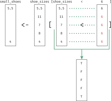
6 is recycled to match the length of the shoe_sizes vector. The resulting boolean values are used to filter the vector.
7.5 Modifying Vectors
Most operations applied to vectors will create a new vector with the modified values. This is the most common process you will use in R. However, it is also possible to manipulate the contents of an existing vector in various ways.
You can assign an element at a particular vector index a new value by specifying the index on the left-hand side of the operation:
# Create a vector `prices`
prices <- c(25, 28, 30)

# Change the first price to 20
prices[1] <- 20
print(prices)
# [1] 20 28 30
To create a new element in your vector, you need to specify the index in which you want to store the new value:
# Create a vector `prices`
prices <- c(25, 28, 30)

# Add a fourth price
prices[4] <- 32

# Add a new price (35) to the end of the vector
new_index <- length(prices) + 1 # the "end" is 1 after the last element
prices[new_index] <- 35
Of course, there’s no reason that you can’t select multiple elements on the left-hand side and assign them multiple values. The assignment operator is also vectorized!
# Create a vector of school supplies
school_supplies <- c("Backpack", "Laptop", "Pen")

# Replace "Laptop" with "Tablet", and "Pen" with "Pencil"
school_supplies[ c(2, 3)] <- c("Tablet", "Pencil")
If you try to modify an element at an index that is greater than the length of the vector, R will fill the vector with NA values:
# Create a vector `prices`
prices <- c(25, 28, 30)

# Set the sixth element in the vector to have the value 60
prices[6] <- 60
print(prices)
# [1] 25 28 30 NA NA 60
Since keeping track of indices can be difficult (and may easily change with your data, making the code fragile), a better approach for adding information at the end of a vector is to create a new vector by combining an existing vector with new elements(s):
# Use the combine (`c()`) function to create a vector
people <- c("Sarah", "Amit", "Zhang")

# Use the `c()` function to combine the `people` vector and the name "Josh"
more_people <- c(people, "Josh")
print(more_people)
# [1] "Sarah" "Amit" "Zhang" "Josh"
Finally, vector modification can be combined with vector filtering to allow you to replace a specific subset of values. For example, you could replace all values in a vector that were greater than 10 with the number 10 (to “cap” the values). Because the assignment operator is vectorized, you can leverage recycling to assign a single value to each element that has been filtered from the vector:
# Create a vector of values
v1 <- c(1, 5, 55, 1, 3, 11, 4, 27)

# Replace all values greater than 10 with 10
v1[v1 > 10] <- 10 # returns 1 5 10 1 3 10 4 10
In this example, the number 10 gets recycled for each element in which v1 is greater than 10 (v1[v1 > 10]).
This technique is particularly powerful when wrangling and cleaning data, as it will allow you to identify and manipulate invalid values or other outliers.
Overall, vectors provide a powerful way of organizing and grouping data for analysis, and will be used throughout your programming with R. For practice working with vectors in R, see the set of accompanying book exercises.2
2Vector exercises: https://github.com/programming-for-data-science/chapter-07-exercises