
11
Manipulating Data with dplyr
The dplyr1 (“dee-ply-er”) package is the preeminent tool for data wrangling in R (and perhaps in data science more generally). It provides programmers with an intuitive vocabulary for executing data management and analysis tasks. Learning and using this package will make your data preparation and management process faster and easier to understand. This chapter introduces the philosophy behind the package and provides an overview of how to use the package to work with data frames using its expressive and efficient syntax.
1dplyr: http://dplyr.tidyverse.org
11.1 A Grammar of Data Manipulation
Hadley Wickham, the original creator of the dplyr package, fittingly refers to it as a Grammar of Data Manipulation. This is because the package provides a set of verbs (functions) to describe and perform common data preparation tasks. One of the core challenges in programming is mapping from questions about a data set to specific programming operations. The presence of a data manipulation grammar makes this process smoother, as it enables you to use the same vocabulary to both ask questions and write your program. Specifically, the dplyr grammar lets you easily talk about and perform tasks such as the following:
Select specific features (columns) of interest from a data set
Filter out irrelevant data and keep only observations (rows) of interest
Mutate a data set by adding more features (columns)
Arrange observations (rows) in a particular order
Summarize data in terms of aggregates such as the mean, median, or maximum
Join multiple data sets together into a single data frame
You can use these words when describing the algorithm or process for interrogating data, and then use dplyr to write code that will closely follow your “plain language” description because it uses functions and procedures that share the same language. Indeed, many real-world questions about a data set come down to isolating specific rows/columns of the data set as the “elements of interest” and then performing a basic comparison or computation (e.g., mean, count, max). While it is possible to perform such computation with base R functions (described in the previous chapters), the dplyr package makes it much easier to write and read such code.
11.2 Core dplyr Functions
The dplyr package provides functions that mirror the verbs mentioned previously. Using this package’s functions will allow you to quickly and effectively write code to ask questions of your data sets.
Since dplyr is an external package, you will need to install it (once per machine) and load it in each script in which you want to use the functions:
install.packages("dplyr") # once per machine
library("dplyr")          # in each relevant script
Fun Fact
dplyr is a key part of thetidyversea collection of R packages, which also includes tidyr (Chapter 12) and ggplot2 (Chapter 16). While these packages are discussed individually, you can install and use them all at once by installing and loading the collected "tidyverse" package.
After loading the package, you can call any of the functions just as if they were the built-in functions you’ve come to know and love.
To demonstrate the usefulness of the dplyr package as a tool for asking questions of real data sets, this chapter applies the functions to historical data about U.S. presidential elections. The presidentialElections data set is included as part of the pscl package, so you will need to install and load that package to access the data:
# Install the `pscl` package to use the `presidentialElections` data frame
install.packages("pscl") # once per machine
library("pscl")          # in each relevant script

# You should now be able to interact with the data set
View(presidentialElections)
This data set contains the percentage of votes that were cast in each state for the Democratic Party candidate in each presidential election from 1932 to 2016. Each row contains the state, year, percentage of Democrat votes (demVote), and whether each state was a member of the former Confederacy during the Civil War (south). For more information, see the pscl package reference manual,2 or use ?presidentialElections to view the documentation in RStudio.
2pscl reference manual: https://cran.r-project.org/web/packages/pscl/pscl.pdf
11.2.1 Select
The select() function allows you to choose and extract columns of interest from your data frame, as illustrated in Figure 11.1.
# Select `year` and `demVotes` (percentage of vote won by the Democrat)
# from the `presidentialElections` data frame
votes <- select(presidentialElections, year, demVote)
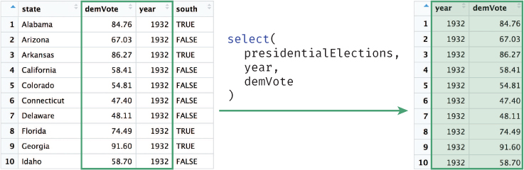
select() function to select the columns year and demVote from the presidentialElections data frame.The select() function takes as arguments the data frame to select from, followed by the names of the columns you wish to select (without quotation marks)!
This use of select() is equivalent to simply extracting the columns using base R syntax:
# Extract columns by name (i.e., "base R" syntax)
votes <- presidentialElections[, c ("year", "demVote")]
While this base R syntax achieves the same end, the dplyr approach provides a more expressive syntax that is easier to read and write.
Remember
Inside the function argument list (inside the parentheses) of dplyr functions, you specify data frame columns without quotation marks—that is, you just give the column names as variable names, rather than as character strings. This is referred to as non-standard evaluation (NSE).a While this capability makes dplyr code easier to write and read, it can occasionally create challenges when trying to work with a column name that is stored in a variable.
If you encounter errors in such situations, you can and should fall back to working with base R syntax (e.g., dollar sign and bracket notation).
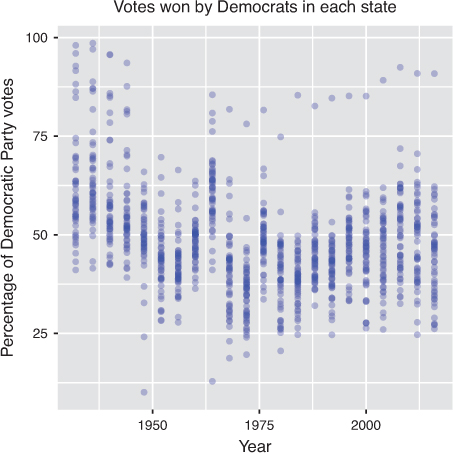
This selection of data could be used to explore trends in voting patterns across states, as shown in Figure 11.2. For an interactive exploration of how state voting patterns have shifted over time, see this piece by the New York Times.3
3Over the Decades, How States Have Shifted: https://archive.nytimes.com/www.nytimes.com/interactive/2012/10/15/us/politics/swing-history.html
ggplot2 package.
Note that the arguments to the select() function can also be vectors of column names—you can write exactly what you would specify inside bracket notation, just without calling c(). Thus you can both select a range of columns using the : operator, and exclude columns using the - operator:
# Select columns `state` through `year` (i.e., `state`, `demVote`, and `year`)
select(presidentialElections, state:year)

# Select all columns except for `south`
select(presidentialElections, -south)
Caution
Unlike with the use of bracket notation, using select() to select a single column will return a data frame, not a vector. If you want to extract a specific column or value from a data frame, you can use the pull() function from the dplyr package, or use base R syntax. In general, use dplyr for manipulating a data frame, and then use base R for referring to specific values in that data.
11.2.2 Filter
The filter() function allows you to choose and extract rows of interest from your data frame (contrasted with select(), which extracts columns), as illustrated in Figure 11.3.
# Select all rows from the 2008 election
votes_2008 <- filter(presidentialElections, year == 2008)

filter() function to select observations from the presidentialElections data frame in which the year column is 2008.
The filter() function takes in the data frame to filter, followed by a comma-separated list of conditions that each returned row must satisfy. Again, column names must be specified without quotation marks. The preceding filter() statement is equivalent to extracting the rows using the following base R syntax:
# Select all rows from the 2008 election
votes_2008 <- presidentialElections[presidentialElections$year == 2008, ]
The filter() function will extract rows that match all given conditions. Thus you can specify that you want to filter a data frame for rows that meet the first condition and the second condition (and so on). For example, you may be curious about how the state of Colorado voted in 2008:
# Extract the row(s) for the state of Colorado in 2008
# Arguments are on separate lines for readability
votes_colorado_2008 <- filter(
  presidentialElections,
  year == 2008,
  state == "Colorado"
)
In cases where you are using multiple conditions—and therefore might be writing really long code—you should break the single statement into multiple lines for readability (as in the preceding example). Because you haven’t closed the parentheses on the function arguments, R will treat each new line as part of the current statement. See the tidyverse style guide4 for more details.
4tidyverse style guide: http://style.tidyverse.org
Caution
If you are working with a data frame that has row names (presidentialElections does not), the dplyr functions will remove row names. If you need to retain these names, consider instead making them a column (feature) of the data, thereby allowing you to include those names in your wrangling and analysis. You can add row names as a column using the mutate function (described in Section 11.2.3):
# Add row names of a dataframe `df` as a new column called `row_names`
df <- mutate(df, row_names = rownames(df))
11.2.3 Mutate
The mutate() function allows you to create additional columns for your data frame, as illustrated in Figure 11.4. For example, it may be useful to add a column to the presidentialElections data frame that stores the percentage of votes that went to other candidates:
# Add an `other_parties_vote` column that is the percentage of votes
# for other parties
# Also add an `abs_vote_difference` column of the absolute difference
# between percentages
# Note you can use columns as you create them!
presidentialElections <- mutate(
  presidentialElections,
  other_parties_vote = 100 - demVote, # other parties is 100% - Democrat %
  abs_vote_difference = abs(demVote - other_parties_vote)
)
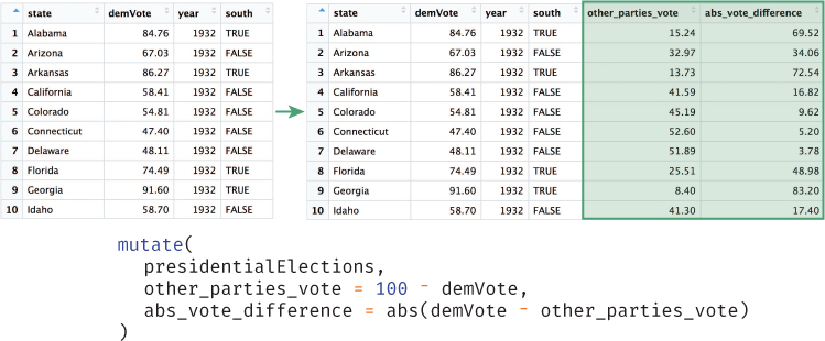
mutate() function to create new columns on the presidentialElections data frame. Note that the mutate() function does not actually change a data frame (you need to assign the result to a variable).
The mutate() function takes in the data frame to mutate, followed by a comma-separated list of columns to create using the same name = vector syntax you use when creating lists or data frames from scratch. As always, the names of the columns in the data frame are specified without quotation marks. Again, it is common to put each new column declaration on a separate line for spacing and readability.
Caution
Despite the name, the mutate() function doesn’t actually change the data frame; instead, it returns a new data frame that has the extra columns added. You will often want to replace your old data frame variable with this new value (as in the preceding code).
Tip
If you want to rename a particular column rather than adding a new one, you can use the dplyr function rename(), which is actually a variation of passing a named argument to the select() function to select columns aliased to different names.
11.2.4 Arrange
The arrange() function allows you to sort the rows of your data frame by some feature (column value), as illustrated in Figure 11.5. For example, you may want to sort the presidentialElections data frame by year, and then within each year, sort the rows based on the percentage of votes that went to the Democratic Party candidate:
# Arrange rows in decreasing order by `year`, then by `demVote`
# within each `year`
presidentialElections <- arrange(presidentialElections, -year, demVote)
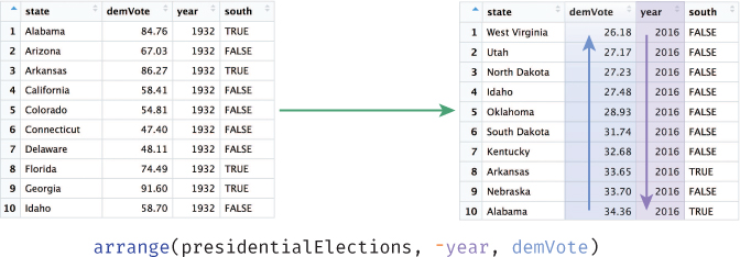
arrange() function to sort the presidentialElections data frame. Data is sorted in decreasing order by year (-year), then sorted by the demVote column within each year.
As demonstrated in the preceding code, you can pass multiple arguments into the arrange() function (in addition to the data frame to arrange). The data frame will be sorted by the column provided as the second argument, then by the column provided as the third argument (in case of a “tie”), and so on. Like mutate(), the arrange() function doesn’t actually modify the argument data frame; instead, it returns a new data frame that you can store in a variable to use later.
By default, the arrange() function will sort rows in increasing order. To sort in reverse (decreasing) order, place a minus sign (-) in front of the column name (e.g., -year). You can also use the desc() helper function; for example, you can pass desc(year) as the argument.
11.2.5 Summarize
The summarize() function (equivalently summarise() for those using the British spelling) will generate a new data frame that contains a “summary” of a column, computing a single value from the multiple elements in that column. This is an aggregation operation (i.e., it will reduce an entire column to a single value—think about taking a sum or average), as illustrated in Figure 11.6. For example, you can calculate the average percentage of votes cast for Democratic Party candidates:
# Compute summary statistics for the `presidentialElections` data frame
average_votes <- summarize(
  presidentialElections,
  mean_dem_vote = mean(demVote),
  mean_other_parties = mean(other_parties_vote)
)
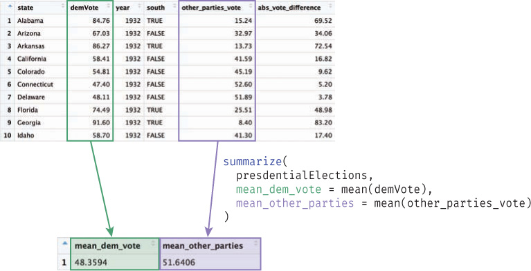
summarize() function to calculate summary statistics for the presidentialElections data frame.
The summarize() function takes in the data frame to aggregate, followed by values that will be computed for the resulting summary table. These values are specified using name = value syntax, similar to using mutate() or defining a list. You can use multiple arguments to include multiple aggregations in the same statement. This will return a data frame with a single row and a different column for each value that is computed by the function, as shown in Figure 11.6.
The summarize() function produces a data frame (a table) of summary values. If you want to reference any of those individual aggregates, you will need to extract them from this table using base R syntax or the dplyr function pull().
You can use the summarize() function to aggregate columns with any function that takes a vector as a parameter and returns a single value. This includes many built-in R functions such as mean(), max(), and median(). Alternatively, you can write your own summary functions. For example, using the presidentialElections data frame, you may want to find the least close election (i.e., the one in which the demVote was furthest from 50% in absolute value). The following code constructs a function to find the value furthest from 50 in a vector, and then applies the function to the presidentialElections data frame using summarize():
# A function that returns the value in a vector furthest from 50
furthest_from_50 <- function(vec) {
  # Subtract 50 from each value
  adjusted_values <- vec - 50

  # Return the element with the largest absolute difference from 50
  vec[ abs(adjusted_values) == max(abs(adjusted_values))]
}

# Summarize the data frame, generating a column `biggest_landslide`
# that stores the value furthest from 50%
summarize(
  presidentialElections,
  biggest_landslide = furthest_from_50(demVote)
)
The true power of the summarize() function becomes evident when you are working with data that has been grouped. In that case, each different group will be summarized as a different row in the summary table (see Section 11.4).
11.3 Performing Sequential Operations
If you want to do more complex analysis, you will likely want to combine these functions, taking the results from one function call and passing them into another function—this is a very common workflow. One approach to performing this sequence of operations is to create intermediary variables for use in your analysis. For example, when working with the presidentialElections data set, you may want to ask a question such as the following:
“Which state had the highest percentage of votes for the Democratic Party candidate (Barack Obama) in 2008?”
Answering this seemingly simple question requires a few steps:
Filter down the data set to only observations from 2008.
Of the percentages in 2008, filter down to the one with the highest percentage of votes for a Democrat.
Select the name of the state that meets the above criteria.
You could then implement each step as follows:
# Use a sequence of steps to find the state with the highest 2008
# `demVote` percentage

# 1. Filter down to only 2008 votes
votes_2008 <- filter(presidentialElections, year == 2008)

# 2. Filter down to the state with the highest `demVote`
most_dem_votes <- filter(votes_2008, demVote == max(demVote))

# 3. Select name of the state
most_dem_state <- select(most_dem_votes, state)
While this approach works, it clutters the work environment with variables you won’t need to use again. It does help with readability (the result of each step is explicit), but those extra variables make it harder to modify and change the algorithm later (you have to change them in two places).
An alternative to saving each step as a distinct, named variable would be to use anonymous variables and nest the desired statements within other functions. While this is possible, it quickly becomes difficult to read and write. For example, you could write the preceding algorithm as follows:
# Use nested functions to find the state with the highest 2008
# `demVote` percentage
most_dem_state <- select(    # 3. Select name of the state
  filter((                   # 2. Filter down to the highest `demVote`
    filter(                  # 1. Filter down to only 2008 votes
      presidentialElections, # arguments for the Step 1 `filter`
      year == 2008
    ),
    demVote == max(demVote)  # second argument for the Step 2 `filter`
  ),
  state                      # second argument for the Step 3 `select`
)
This version uses anonymous variables—result values that are not assigned to variables (and so are anonymous)—but instead are immediately used as the arguments to other functions. You’ve used these anonymous variables frequently with the print() function and with filters (those vectors of TRUE and FALSE values)—even the max(demVote) in the Step 2 filter is an anonymous variable!
This nested approach achieves the same result as the previous example does without creating extra variables. But, even with only three steps, it can get quite complicated to read—in a large part because you have to think about it “inside out,” with the code in the middle being evaluated first. This will obviously become undecipherable for more involved operations.
11.3.1 The Pipe Operator
Luckily, dplyr provides a cleaner and more effective way of performing the same task (that is, using the result of one function as an argument to the next). The pipe operator (written as %>%) takes the result from one function and passes it in as the first argument to the next function! You can answer the question asked earlier much more directly using the pipe operator as follows:
# Ask the same question of our data using the pipe operator
most_dem_state <- presidentialElections %>% # data frame to start with
  filter(year == 2008) %>% # 1. Filter down to only 2008 votes
  filter(demVote == max(demVote)) %>% # 2. Filter down to the highest `demVote`
  select(state) # 3. Select name of the state
Here the presidentialElections data frame is “piped” in as the first argument to the first filter() call; because the argument has been piped in, the filter() call takes in only the remaining arguments (e.g., year == 2008). The result of that function is then piped in as the first argument to the second filter() call (which needs to specify only the remaining arguments), and so on. The additional arguments (such as the filter criteria) continue to be passed in as normal, as if no data frame argument is needed.
Because all dplyr functions discussed in this chapter take as a first argument the data frame to manipulate, and then return a manipulated data frame, it is possible to “chain” together any of these functions using a pipe!
Yes, the %>% operator can be awkward to type and takes some getting use to (especially compared to the command line’s use of | to pipe). However, you can ease the typing by using the RStudio keyboard shortcut cmd+shift+m.
Tip
You can see all RStudio keyboard shortcuts by navigating to the Tools > Keyboard Shortcuts Help menu, or you can use the keyboard shortcut alt+shift+k (yes, this is the keyboard shortcut to show the keyboard shortcuts menu!).
The pipe operator is loaded when you load the dplyr package (it is available only if you load that package), but it will work with any function, not just dplyr ones. This syntax, while slightly odd, can greatly simplify the way you write code to ask questions about your data.
Fun Fact
Many packages load other packages (which are referred to as dependencies). For example, the pipe operator is actually part of the magrittra package, which is loaded as a dependency of dplyr.
ahttps://cran.r-project.org/web/packages/magrittr/vignettes/magrittr.html
Note that as in the preceding example, it is best practice to put each “step” of a pipe sequence on its own line (indented by two spaces). This allows you to easily rearrange the steps (simply by moving lines), as well as to “comment out” particular steps to test and debug your analysis as you go.
11.4 Analyzing Data Frames by Group
dplyr functions are powerful, but they are truly awesome when you can apply them to groups of rows within a data set. For example, the previously described use of summarize() isn’t particularly useful since it just gives a single summary for a given column (which you could have done easily using base R functions). However, a grouped operation would allow you to compute the same summary measure (e.g., mean, median, sum) automatically for multiple groups of rows, enabling you to ask more nuanced questions about your data set.
The group_by() function allows you to create associations among groups of rows in a data frame so that you can easily perform such aggregations. It takes as arguments a data frame to do the grouping on, followed by which column(s) you wish to use to group the data—each row in the table will be grouped with other rows that have the same value in that column. For example, you can group all of the data in the presidentialElections data set into groups whose rows share the same state value:
# Group observations by state
grouped <- group_by(presidentialElections, state)
The group_by() function returns a tibble,5 which is a version of a data frame used by the “tidyverse”6 family of packages (which includes dplyr). You can think of this as a “special” kind of data frame—one that is able to keep track of “subsets” (groups) within the same variable. While this grouping is not visually apparent (i.e., it does not sort the rows), the tibble keeps track of each row’s group for computation, as shown in Figure 11.7.
5tibble package website: http://tibble.tidyverse.org
6tidyverse website: https://www.tidyverse.org

group_by() function—that stores associations by the grouping variable (state). Red notes are added.
The group_by() function is useful because it lets you apply operations to groups of data without having to explicitly break your data into different variables (sometimes called bins or chunks). Once you’ve used group_by() to group the rows of a data frame, you can apply other verbs (e.g., summarize(), filter()) to that tibble, and they will be automatically applied to each group (as if they were separate data frames). Rather than needing to explicitly extract different sets of data into separate data frames and run the same operations on each, you can use the group_by() function to accomplish all of this with a single command:
# Compute summary statistics by state: average percentages across the years
state_voting_summary <- presidentialElections %>%
  group_by(state) %>%
  summarize(
    mean_dem_vote = mean(demVote),
    mean_other_parties = mean(other_parties_vote)
  )
The preceding code will first group the rows together by state, then compute summary information (mean() values) for each one of these groups (i.e., for each state), as illustrated in Figure 11.8. A summary of groups will still return a tibble, where each row is the summary of a different group. You can extract values from a tibble using dollar sign or bracket notation, or convert it back into a normal data frame with the as.data.frame() function.
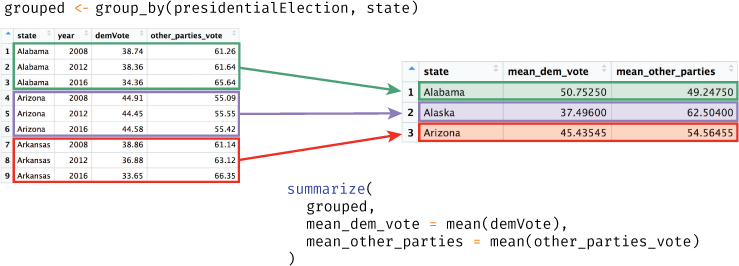
group_by() and summarize() functions to calculate summary statistics in the presidentialElections data frame by state.
This form of grouping can allow you to quickly compare different subsets of your data. In doing so, you’re redefining your unit of analysis. Grouping lets you frame your analysis question in terms of comparing groups of observations, rather than individual observations. This form of abstraction makes it easier to ask and answer complex questions about your data.
11.5 Joining Data Frames Together
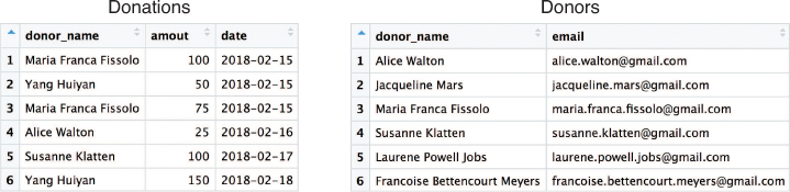
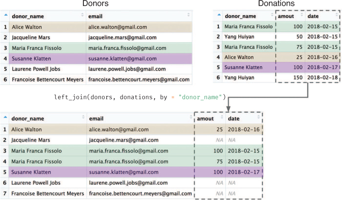
When working with real-world data, you will often find that the data is stored across multiple files or data frames. This can be done for a number of reasons, such as reducing memory usage. For example, if you had a data frame containing information on a fundraising campaign that tracked donations (e.g., dollar amount, date), you would likely store information about each donor (e.g., email, phone number) in a separate data file (and thus data frame). See Figure 11.9 for an example of what this structure would look like.
This structure has a number of benefits:
Data storage: Rather than duplicating information about each donor every time that person makes a donation, you can store that information a single time. This will reduce the amount of space your data takes up.
Data updates: If you need to update information about a donor (e.g., the donor’s phone number changes), you can make that change in a single location.
This separation and organization of data is a core concern in the design of relational databases, which are discussed in Chapter 13.
At some point, you will want to access information from both data sets (e.g., you need to email donors about their contributions), and thus need a way to reference values from both data frames at once—in effect, to combine the data frames. This process is called a join (because you are “joining” the data frames together). When you perform a join, you identify columns which are present in both tables, and use those columns to “match” corresponding rows to one another. Those column values are used as identifiers to determine which rows in each table correspond to one another, and thus will be combined into a single row in the resulting (joined) table.
The left_join() function is one example of a join. This function looks for matching columns between two data frames, and then returns a new data frame that is the first (“left”) argument with extra columns from the second (“right”) argument added on—in effect, “merging” the tables. You specify which columns you want to “match” on by specifying a by argument, which takes a vector of columns names (as strings).
For example, because both of the data frames in Figure 11.9 have a donor_name column, you can “match” the rows from the donor table to the donations table by this column and merge them together, producing the joined table illustrated in Figure 11.10.
# Combine (join) donations and donors data frames by their shared column
# ("donor_name")
combined_data <- left_join(donations, donors, by = "donor_name")
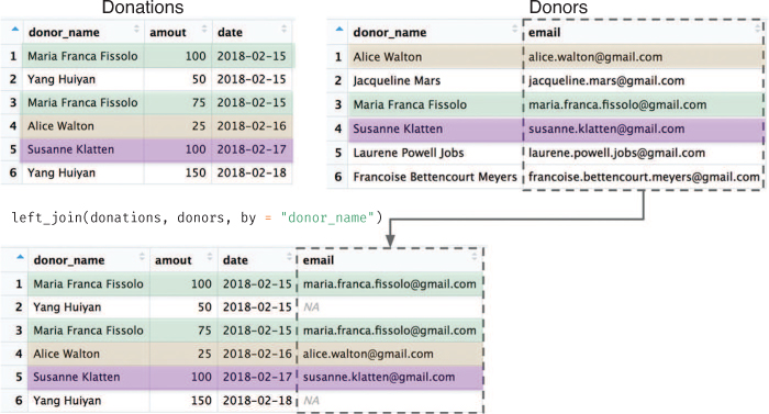
Donors) are added to the end of the left-hand table (Donations). Rows are on matched on the shared column (donor_name). Note the observations present in the left-hand table that don’t have a corresponding row in the right-hand table (Yang Huiyan).
When you perform a left join as in the preceding code, the function performs the following steps:
It goes through each row in the table on the “left” (the first argument; e.g.,
donations), considering the values from the shared columns (e.g.,donor_name).For each of these values from the left-hand table, the function looks for a row in the right-hand table (e.g.,
donors) that has the same value in the specified column.If it finds such a matching row, it adds any other data values from columns that are in
donorsbut not indonationsto that left-hand row in the resulting table.It repeats steps 1–3 for each row in the left-hand table, until all rows have been given values from their matches on the right (if any).
You can see in Figure 11.10 that there were elements in the left-hand table (donations) that did not match to a row in the right-hand table (donors). This may occur because there are some donations whose donors do not have contact information (there is no matching donor_name entry): those rows will be given NA (not available) values, as shown in Figure 11.10.
Remember
A left join returns all of the rows from the first table, with all of the columns from both tables.
For rows to match, they need to have the same data in all specified shared columns. However, if the names of your columns don’t match or if you want to match only on specific columns, you can use a named vector (one with tags similar to a list) to indicate the different names from each data frame. If you don’t specify a by argument, the join will match on all shared column names.
# An example join in the (hypothetical) case where the tables have
# different identifiers; e.g., if `donations` had a column `donor_name`,
# while `donors` had a column `name`
combined_data <- left_join(donations, donors, by = c("donor_name" = "name"))
Caution
Because of how joins are defined, the argument order matters! For example, in a left_join(), the resulting table has rows for only the elements in the left (first) table; any unmatched elements in the second table are lost.
If you switch the order of the arguments, you will instead keep all of the information from the donors data frame, adding in available information from donations (see Figure 11.11).
# Combine (join) donations and donors data frames (see Figure 11.11)
combined_data <- left_join(donors, donations, by = "donor_name")
donors) are returned with additional columns from the right-hand table (donations).
Since some donor_name values show up multiple times in the right-hand (donations) table, the rows from donors end up being repeated so that the information can be “merged” with each set of values from donations. Again, notice that rows that lack a match in the right-hand table don’t get any additional information (representing “donors” who gave their contact information to the organization, but have not yet made a donation).
Because the order of the arguments matters, dplyr (and relational database systems in general) provide several different kinds of joins, each influencing which rows are included in the final table. Note that in all joins, columns from both tables will be present in the resulting table—the join type dictates which rows are included. See Figure 11.12 for a diagram of these joins.
left_join: All rows from the first (left) data frame are returned. That is, you get all the data from the left-hand table, with extra column values added from the right-hand table. Left-hand rows without a match will haveNAin the right-hand columns.right_join: All rows from the second (right) data frame are returned. That is, you get all the data from the right-hand table, with extra column values added from the left-hand table. Right-hand rows without a match will haveNAin the left-hand columns. This is the “opposite” of aleft_join, and the equivalent of switching the order of the arguments.inner_join: Only rows in both data frames are returned. That is, you get any rows that had matching observations in both tables, with the column values from both tables. There will be no additionalNAvalues created by the join. Observations from the left that had no match in the right, or observations from the right that had no match in the left, will not be returned at all—the order of arguments does not matter.full_join: All rows from both data frames are returned. That is, you get a row for any observation, whether or not it matched. If it happened to match, values from both tables will appear in that row. Observations without a match will haveNAin the columns from the other table—the order of arguments does not matter.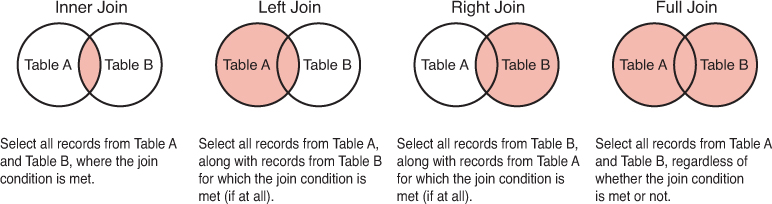
Figure 11.12 A diagram of different join types, downloaded from http://www.sql-join.com/sql-join-types/.
The key to deciding between these joins is to think about which set of data you want as your set of observations (rows), and which columns you’d be okay with being NA if a record is missing.
Tip
Jenny Bryan has created an excellent “cheatsheet”a for dplyr join functions that you can reference.
11.6 dplyr in Action: Analyzing Flight Data
In this section, you will learn how dplyr functions can be used to ask interesting questions of a more complex data set (the complete code for this analysis is also available online in the book’s code repository7). You’ll use a data set of flights that departed from New York City airports (including Newark, John F. Kennedy, and Laguardia airports) in 2013. This data set is also featured online in the Introduction to dplyr vignette,8 and is drawn from the Bureau of Transportation Statistics database.9 To load the data set, you will need to install and load the nycflights13 package. This will load the flights data set into your environment.
7dplyr in Action: https://github.com/programming-for-data-science/in-action/tree/master/dplyr
8Introduction to dplyr: http://dplyr.tidyverse.org/articles/dplyr.html
9Bureau of Labor Statistics: air flights data: https://www.transtats.bts.gov/DatabaseInfo.asp?DB_ID=120
# Load the `nycflights13` package to access the `flights` data frame
install.packages("nycflights13") # once per machine
library("nycflights13")          # in each relevant script
Before you can start asking targeted questions of the data set, you will need to understand the structure of the data set a bit better:
# Getting to know the `flights` data set
?flights          # read the available documentation
dim(flights)      # check the number of rows/columns
colnames(flights) # inspect the column names
View(flights)     # look at the data frame in the RStudio Viewer
A subset of the flights data frame in RStudio’s Viewer is shown in Figure 11.13.
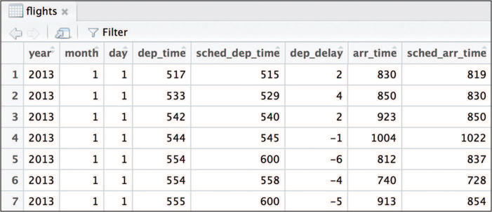
flights data set, which is included as part of the nycflights13 package.Given this information, you may be interested in asking questions such as the following:
Which airline has the highest number of delayed departures?
On average, to which airport do flights arrive most early?
In which month do flights tend to have the longest delays?
Your task here is to map from these questions to specific procedures so that you can write the appropriate dplyr code.
You can begin by asking the first question:
“Which airline has the highest number of delayed departures?”
This question involves comparing observations (flights) that share a particular feature (airline), so you perform the analysis as follows:
Since you want to consider all the flights from a particular airline (based on the
carrierfeature), you will first want to group the data by that feature.You need to figure out the largest number of delayed departures (based on the
dep_delayfeature)—which means you need to find the flights that were delayed (filtering for them).You can take the found flights and aggregate them into a count (summarize the different groups).
You will then need to find which group has the highest count (filtering).
Finally, you can choose (select) the airline of that group.
Tip
When you’re trying to find the right operation to answer your question of interest, the phrase “Find the entry that…” usually corresponds to a filter() operation!
Once you have established this algorithm, you can directly map it to dplyr functions:
# Identify the airline (`carrier`) that has the highest number of
# delayed flights
has_most_delays <- flights %>%            # start with the flights
  group_by(carrier) %>%                   # group by airline (carrier)
  filter(dep_delay > 0) %>%               # find only the delays
  summarize(num_delay = n()) %>%          # count the observations
  filter(num_delay == max(num_delay)) %>% # find most delayed
  select(carrier)                         # select the airline
Remember
Often many approaches can be used to solve the same problem. The preceding code shows one possible approach; as an alternative, you could filter for delayed departures before grouping. The point is to think through how you might solve the problem (by hand) in terms of the Grammar of Data Manipulation, and then convert that into dplyr!
Unfortunately, the final answer to this question appears to be an abbreviation: UA. To reduce the size of the flights data frame, information about each airline is stored in a separate data frame called airlines. Since you are interested in combining these two data frames (your answer and the airline information), you can use a join:
# Get name of the most delayed carrier
most_delayed_name <- has_most_delays %>%  # start with the previous answer
  left_join(airlines, by = "carrier") %>% # join on airline ID
  select(name)                            # select the airline name

print(most_delayed_name$name) # access the value from the tibble
# [1] "United Air Lines Inc."
After this step, you will have learned that the carrier that had the largest absolute number of delays was United Air Lines Inc. Before criticizing the airline too strongly, however, keep in mind that you might be interested in the proportion of flights that are delayed, which would require a separate analysis.
Next, you can assess the second question:
“On average, to which airport do flights arrive most early?”
To answer this question, you can follow a similar approach. Because this question pertains to how early flights arrive, the outcome (feature) of interest is arr_delay (noting that a negative amount of delay indicates that the flight arrived early). You will want to group this information by destination airport (dest) where the flight arrived. And then, since you’re interested in the average arrival delay, you will want to summarize those groups to aggregate them:
# Calculate the average arrival delay (`arr_delay`) for each destination
# (`dest`)
most_early <- flights %>%
  group_by(dest) %>% # group by destination
  summarize(delay = mean(arr_delay)) # compute mean delay
It’s always a good idea to check your work as you perform each step of an analysis—don’t write a long sequence of manipulations and hope that you got the right answer! By printing out the most_early data frame at this point, you notice that it has a lot of NA values, as seen in Figure 11.14.
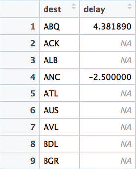
flights data set. Because NA values are present in the data set, the mean delay for many destinations is calculated as NA. To remove NA values from the mean() function, set na.rm = FALSE.
This kind of unexpected result occurs frequently when doing data programming—and the best way to solve the problem is to work backward. By carefully inspecting the arr_delay column, you may notice that some entries have NA values—the arrival delay is not available for that record. Because you can’t take the mean() of NA values, you decide to exclude those values from the analysis. You can do this by passing an na.rm = TRUE argument (“NA remove”) to the mean() function:
# Compute the average delay by destination airport, omitting NA results
most_early <- flights %>%
  group_by(dest) %>% # group by destination
  summarize(delay = mean(arr_delay, na.rm = TRUE)) # compute mean delay
Removing NA values returns numeric results, and you can continue working through your algorithm:
# Identify the destination where flights, on average, arrive most early
most_early <- flights %>%
  group_by(dest) %>% # group by destination
  summarize(delay = mean(arr_delay, na.rm = TRUE)) %>% # compute mean delay
  filter(delay == min(delay, na.rm = TRUE)) %>% # filter for least delayed
  select(dest, delay) %>% # select the destination (and delay to store it)
  left_join(airports, by = c("dest" = "faa")) %>% # join on `airports` data
  select(dest, name, delay) # select output variables of interest

print(most_early)
# A tibble: 1 x 3
#  dest  name       delay
#  <chr> <chr>      <dbl>
#1 LEX   Blue Grass   -22
Answering this question follows a very similar structure to the first question. The preceding code reduces the steps to a single statement by including the left_join() statement in the sequence of piped operations. Note that the column containing the airport code has a different name in the flights and airports data frames (dest and faa, respectively), so you use a named vector value for the by argument to specify the match.
As a result, you learn that LEX—Blue Grass Airport in Lexington, Kentucky—is the airport with the earliest average arrival time (22 minutes early!).
A final question is:
“In which month do flights tend to have the longest delays?”
These kinds of summary questions all follow a similar pattern: group the data by a column (feature) of interest, compute a summary value for (another) feature of interest for each group, filter down to a row of interest, and select the columns that answer your question:
# Identify the month in which flights tend to have the longest delays
flights %>%
  group_by(month) %>% # group by selected feature
  summarize(delay = mean(arr_delay, na.rm = TRUE)) %>% # summarize delays
  filter(delay == max(delay)) %>% # filter for the record of interest
  select(month) %>% # select the column that answers the question
  print() # print the tibble out directly
# A tibble: 1 x 1
#  month
#  <int>
#1   7
If you are okay with the result being in the form of a tibble rather than a vector, you can even pipe the results directly to the print() function to view the results in the R console (the answer being July). Alternatively, you can use a package such as ggplot2 (see Chapter 16) to visually communicate the delays by month, as in Figure 11.15.
# Compute delay by month, adding month names for visual display
# Note, `month.name` is a variable built into R
delay_by_month <- flights %>%
  group_by(month) %>%
  summarize(delay = mean(arr_delay, na.rm = TRUE)) %>%
  select(delay) %>%
  mutate(month = month.name)

# Create a plot using the ggplot2 package (described in Chapter 17)
ggplot(data = delay_by_month) +
  geom_point(
    mapping = aes(x = delay, y = month),
    color = "blue",
    alpha = .4,
    size = 3
  ) +
  geom_vline(xintercept = 0, size = .25) +
  xlim(c(-20, 20)) +
  scale_y_discrete(limits = rev(month.name)) +
  labs(title = "Average Delay by Month", y = "", x = "Delay (minutes)")

flights data set. The plot is built using ggplot2 (discussed in Chapter 16).
Overall, understanding how to formulate questions, translate them into data manipulation steps (following the Grammar of Data Manipulation), and then map those to dplyr functions will enable you to quickly and effectively learn pertinent information about your data set. For practice wrangling data with the dplyr package, see the set of accompanying book exercises.10
10dplyr exercises: https://github.com/programming-for-data-science/chapter-11-exercises