13
Accessing Databases
This chapter introduces relational databases as a way to structure and organize complex data sets. After introducing the purpose and format of relational databases, it describes the syntax for interacting with them using R. By the end of the chapter you will be able to wrangle data from a database.
13.1 An Overview of Relational Databases
Simple data sets can be stored and loaded from .csv files, and are readily represented in the computer’s memory as a data frame. This structure works great for data that is structured just as a set of observations made up of features. However, as data sets become more complex, you run against some limitations.
In particular, your data may not be structured in a way that it can easily and efficiently be represented as a single data frame. For example, imagine you were trying to organize information about music playlists (e.g., on a service such as Spotify). If your playlist is the unit of analysis you are interested in, each playlist would be an observation (row) and would have different features (columns) included. One such feature you could be interested in is the songs that appear on the playlist (implying that one of your columns should be songs). However, playlists may have lots of different songs, and you may also be tracking further information about each song (e.g., the artist, the genre, the length of the song). Thus you could not easily represent each song as a simple data type such as a number or string. Moreover, because the same song may appear in multiple playlists, such a data set would include a lot of duplicate information (e.g., the title and artist of the song).
To solve this problem, you could use multiple data frames (perhaps loaded from multiple .csv files), joining those data frames together as described in Chapter 11 to ask questions of the data. However, that solution would require you to manage multiple different .csv files, as well as to determine an effective and consistent way of joining them together. Since organizing, tracking, and updating multiple .csv files can be difficult, many large data sets are instead stored in databases. Metonymically, a database is a specialized application (called a database management system) used to save, organize, and access information—similar to what git does for versions of code, but in this case for the kind of data that might be found in multiple .csv files. Because many organizations store their data in a database of some kind, you will need to be able to access that data to analyze it. Moreover, accessing data directly from a database makes it possible to process data sets that are too large to fit into your computer’s memory (RAM) at once. The computer will not be required to hold a reference to all the data at once, but instead will be able to apply your data manipulation (e.g., selecting and filtering the data) to the data stored on a computer’s hard drive.
13.1.1 What Is a Relational Database?
The most commonly used type of database is a relational database. A relational database organizes data into tables similar in concept and structure to a data frame. In a table, each row (also called a record) represents a single “item” or observation, while each column (also called a field) represents an individual data property of that item. In this way, a database table mirrors an R data frame; you can think of them as somewhat equivalent. However, a relational database may be made up of dozens, if not hundreds or even thousands, of different tables—each one representing a different facet of the data. For example, one table may store information about which music playlists are in the database, another may store information about the individual songs, another may store information about the artists, and so on.
What makes relational databases special is how they specify the relationships between these tables. In particular, each record (row) in a table is given a field (column) called the primary key. The primary key is a unique value for each row in the table, so it lets you refer to a particular record. Thus even if there were two songs with the same name and artist, you could still distinguish between them by referencing them through their primary key. Primary keys can be any unique identifier, but they are almost always numbers and are frequently automatically generated and assigned by the database. Note that databases can’t just use the “row number” as the primary key, because records may be added, removed, or reordered—which means a record won’t always be at the same index!
Moreover, each record in one table may be associated with a record in another—for example, each record in a songs table might have an associated record in the artists table indicating which artist performed the song. Because each record in the artists table has a unique key, the songs table is able to establish this association by including a field (column) for each record that contains the corresponding key from artists (see Figure 13.1). This is known as a foreign key (it is the key from a “foreign” or other table). Foreign keys allow you to join tables together, similar to how you would with dplyr. You can think of foreign keys as a formalized way of defining a consistent column for the join() function’s by argument.

id. The songs table (top right) also has an artist_id foreign key used to associate it with the artists table (top left). The bottom table illustrates how the foreign key can be used when joining the tables.
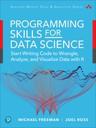
Databases can use tables with foreign keys to organize data into complex structures; indeed, a database may have a table that just contains foreign keys to link together other tables! For example, if a database needs to represent data such that each playlist can have multiple songs, and songs can be on many playlists (a “many-to-many” relationship), you could introduce a new “bridge table” (e.g., playlists_songs) whose records represent the associations between the two other tables (see Figure 13.2). You can think of this as a “table of lines to draw between the other tables.” The database could then join all three of the tables to access the information about all of the songs for a particular playlist.
Going Further
13.1.2 Setting Up a Relational Database
To use a relational database on your own computer (e.g., for experimenting or testing your analysis), you will need to install a separate software program to manage that database. This program is called a relational database management system (RDMS). There are a couple of different popular RDMS systems; each of them provides roughly the same syntax (called SQL) for manipulating the tables in the database, though each may support additional specialized features. The most popular RDMSs are described here. You are not required to install any of these RDMSs to work with a database through R; see Section 13.3, below. However, brief installation notes are provided for your reference.
SQLite1 is the simplest SQL database system, and so is most commonly used for testing and development (though rarely in real-world “production” systems). SQLite databases have the advantage of being highly self-contained: each SQLite database is a single file (with the
.sqliteextension) that is formatted to enable the SQLite RDMS to access and manipulate its data. You can almost think of these files as advanced, efficient versions of.csvfiles that can hold multiple tables! Because the database is stored in a single file, this makes it easy to share databases with others or even place one under version control.1SQLite: https://www.sqlite.org/index.html
To work with an SQLite database you can download and install a command line application2 for manipulating the data. Alternatively, you can use an application such as DB Browser for SQLite,3 which provides a graphical interface for interacting with the data. This is particularly useful for testing and verifying your SQL and
Rcode.2SQLite download page: https://www.sqlite.org/download.html; look for “Precompiled Binaries” for your system.
3DB Browser for SQLite: http://sqlitebrowser.org
PostgreSQL4 (often shortened to “Postgres”) is a free open source RDMS, providing a more robust system and set of features (e.g., for speeding up data access and ensuring data integrity) and functions than SQLite. It is often used in real-world production systems, and is the recommended system to use if you need a “full database.” Unlike with SQLite, a Postgres database is not isolated to a single file that can easily be shared, though there are ways to export a database.
4PostgreSQL: https://www.postgresql.org
You can download and install the Postgres RDMS from its website;5 follow the instructions in the installation wizard to set up the database system. This application will install the manager on your machine, as well as provide you with a graphical application (pgAdmin) to administer your databases. You can also use the provided
psqlcommand line application if you add it to your PATH; alternatively, the SQL Shell application will open the command line interface directly.5PostgreSQL download page: https://www.postgresql.org/download
MySQL6 is a free (but closed source) RDMS, providing a similar level of features and structure as Postgres. MySQL is a more popular system than Postgres, so its use is more common, but can be somewhat more difficult to install and set up.
6MySQL: https://www.mysql.com
If you wish to set up and use a MySQL database, we recommend that you install the Community Server Edition from the MySQL website.7 Note that you do not need to sign up for an account (click the smaller “No thanks, just start my download” link instead).
7MySQL download Page: https://dev.mysql.com/downloads/mysql
We suggest you use SQLite when you’re just experimenting with a database (as it requires the least amount of setup), and recommend Postgres if you need something more full-featured.
13.2 A Taste of SQL
The reason all of the RDMSs described in Section 13.1.2 have “SQL” in their names is because they all use the same syntax—SQL—for manipulating the data stored in the database. SQL (Structured Query Language) is a programming language used specifically for managing data in a relational database—a language that is structured for querying (accessing) that information. SQL provides a relatively small set of commands (referred to as statements), each of which is used to interact with a database (similar to the operations described in the Grammar of Data Manipulation used by dplyr).
This section introduces the most basic of SQL statements: the SELECT statement used to access data. Note that it is absolutely possible to access and manipulate a database through R without using SQL; see Section 13.3. However, it is often useful to understand the underlying commands that R is issuing. Moreover, if you eventually need to discuss database manipulations with someone else, this language will provide some common ground.
Caution
Most RDMSs support SQL, though systems often use slightly different “flavors” of SQL. For example, data types may be named differently, or different RDMSs may support additional functions or features.
Tip
For a more thorough introduction to SQL, w3schoolsa offers a very newbie-friendly tutorial on SQL syntax and usage. You can also find more information in Forta, Sams Teach Yourself SQL in 10 Minutes, Fourth Edition (Sams, 2013), and van der Lans, Introduction to SQL, Fourth Edition (Addison-Wesley, 2007).
The most commonly used SQL statement is the SELECT statement. The SELECT statement is used to access and extract data from a database (without modifying that data)—this makes it a query statement. It performs the same work as the select() function in dplyr. In its simplest form, the SELECT statement has the following format:
/* A generic SELECT query statement for accessing data */
SELECT column FROM table
(In SQL, comments are written on their own line surrounded by /* */.)
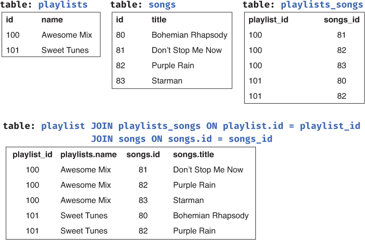
This query will return the data from the specified column in the specified table (keywords like SELECT in SQL are usually written in all-capital letters—though they are not case-sensitive—while column and table names are often lowercase). For example, the following statement would return all of the data from the title column of the songs table (as shown in Figure 13.3):
/* Access the `title` column from the `songs` table */
SELECT title FROM songs
SELECT statement and results shown in the SQLite Browser.
This would be equivalent to select(songs, title) when using dplyr.
You can select multiple columns by separating the names with commas (,). For example, to select both the id and title columns from the songs table, you would use the following query:
/* Access the `id` and `title` columns from the `songs` table */
SELECT id, title FROM songs
If you wish to select all the columns, you can use the special * symbol to represent “everything”—the same wildcard symbol you use on the command line! The following query will return all columns from the songs table:
/* Access all columns from the `songs` table */
SELECT * FROM songs
Using the * wildcard to select data is common practice when you just want to load the entire table from the database.
You can also optionally give the resulting column a new name (similar to a mutate manipulation) by using the AS keyword. This keyword is placed immediately after the name of the column to be aliased, followed by the new column name. It doesn’t actually change the table, just the label of the resulting “subtable” returned by the query.
/* Access the `id` column (calling it `song_id`) from the `songs` table */
SELECT id AS song_id FROM songs
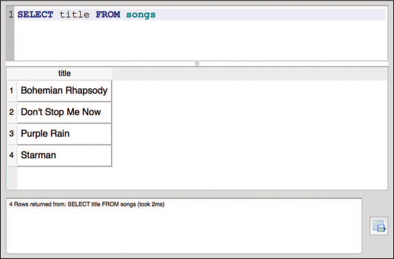
The SELECT statement performs a select data manipulation. To perform a filter manipulation, you add a WHERE clause at the end of the SELECT statement. This clause includes the keyword WHERE followed by a condition, similar to the boolean expression you would use with dplyr. For example, to select the title column from the songs table with an artist_id value of 11, you would use the following query (also shown in Figure 13.4):
/* Access the `title` column from the `songs` table if `artist_id` is 11 */
SELECT title FROM songs WHERE artist_id = 11
WHERE clause and results shown in the SQLite Browser.
This would be the equivalent to the following dplyr statement:
# Filter for the rows with a particular `artist_id`, and then select
# the `title` column
filter(songs, artist_id == 11)  %>%
  select(title)
The filter condition is applied to the whole table, not just the selected columns. In SQL, the filtering occurs before the selection.
Note that a WHERE condition uses = (not ==) as the “is equal” operator. Conditions can also use other relational operators (e.g., >, <=), as well as some special keywords such as LIKE, which will check whether the column value is inside a string. (String values in SQL must be specified in quotation marks—it’s most common to use single quotes.)
You can combine multiple WHERE conditions by using the AND, OR, and NOT keywords as boolean operators:
/* Access all columns from `songs` where EITHER condition applies */
SELECT * FROM songs WHERE artist_id = 12 OR title = 'Starman'
The statement SELECT columns FROM table WHERE conditions is the most common form of SQL query. But you can also include other keyword clauses to perform further data manipulations. For example, you can include an ORDER_BY clause to perform an arrange manipulation (by a specified column), or a GROUP_BY clause to perform aggregation (typically used with SQL-specific aggregation functions such as MAX() or MIN()). See the official documentation for your database system (e.g., for Postgres8) for further details on the many options available when specifying SELECT queries.
8PostgreSQL: SELECT: https://www.postgresql.org/docs/current/static/sql-select.html
The SELECT statements described so far all access data in a single table. However, the entire point of using a database is to be able to store and query data across multiple tables. To do this, you use a join manipulation similar to that used in dplyr. In SQL, a join is specified by including a JOIN clause, which has the following format:
/* A generic JOIN between two tables */
SELECT columns FROM table1 JOIN table2
As with dplyr, an SQL join will by default “match” columns if they have the same value in the same column. However, tables in databases often don’t have the same column names, or the shared column name doesn’t refer to the same value—for example, the id column in artists is for the artist ID, while the id column in songs is for the song ID. Thus you will almost always include an ON clause to specify which columns should be matched to perform the join (writing the names of the columns separated by an = operator):
/* Access artists, song titles, and ID values from two JOINed tables */
SELECT artists.id, artists.name, songs.id, songs.title FROM artists
    JOIN songs ON songs.artist_id = artists.id
This query (shown in Figure 13.5) will select the IDs, names, and titles from the artists and songs tables by matching to the foreign key (artist_id); the JOIN clause appears on its own line just for readability. To distinguish between columns with the same name from different tables, you specify each column first by its table name, followed by a period (.), followed by the column name. (The dot can be read like “apostrophe s” in English, so artists.id would be “the artists table’s id.”)

JOIN statement and results shown in the SQLite Browser.
You can join on multiple conditions by combining them with AND clauses, as with multiple WHERE conditions.
Like dplyr, SQL supports four kinds of joins (see Chapter 11 to review them). By default, the JOIN statement will perform an inner join—meaning that only rows that contain matches in both tables will be returned (e.g., the joined table will not have rows that don’t match). You can also make this explicit by specifying the join clause with the keywords INNER JOIN. Alternatively, you can specify that you want to perform a LEFT JOIN, RIGHT JOIN, or OUTER JOIN (i.e., a full join). For example, to perform a left join you would use a query such as the following:
/* Access artists and song titles, including artists without any songs */
SELECT artists.id, artists.name, songs.id, songs.title FROM artists
    LEFT JOIN songs ON songs.artist_id = artists.id
Notice that the statement is written the same way as before, except with an extra word to clarify the type of join.
As with dplyr, deciding on the type of join to use requires that you carefully consider which observations (rows) must be included, and which features (columns) must not be missing in the table you produce. Most commonly you are interested in an inner join, which is why that is the default!
13.3 Accessing a Database from R
SQL will allow you to query data from a database; however, you would have to execute such commands through the RDMS itself (which provides an interpreter able to understand the syntax). Luckily, you can instead use R packages to connect to and query a database directly, allowing you to use the same, familiar R syntax and data structures (i.e., data frames) to work with databases. The simplest way to access a database through R is to use the dbplyr9 package, which was developed as part of the tidyverse collection. This package allows you to query a relational database using dplyr functions, avoiding the need to use an external application!
9dbplyr repository page: https://github.com/tidyverse/dbplyr
Going Further
Because dbplyr is another external package (like dplyr and tidyr), you will need to install it before you can use it. However, because dbplyr is actually a “backend” for dplyr (it provides the behind-the-scenes code that dplyr uses to work with a database), you actually need to use functions from dplyr and so load in the dplyr package instead. However, you will also need to load the DBI package, which is installed along with dbplyr and allows you to connect to the database:
install.packages("dbplyr") # once per machine
library("DBI")             # in each relevant script
library("dplyr")           # need dplyr to use its functions on the database!
You will also need to install an additional package depending on which kind of database you wish to access. These packages provide a common interface (set of functions) across multiple database formats—they will allow you to access an SQLite database and a Postgres database using the same R functions.
# To access an SQLite database
install.packages("RSQLite") # once per machine
library("RSQLite")          # in each relevant script

# To access a Postgres database
install.packages("RPostgreSQL") # once per machine
library("RPostgreSQL")          # in each relevant script
Remember that databases are managed and accessed through an RDMS, which is a separate program from the R interpreter. Thus, to access databases through R, you will need to “connect” to that external RDMS program and use R to issue statements through it. You can connect to an external database using the dbConnect() function provided by the DBI package:
# Create a "connection" to the RDMS
db_connection <- dbConnect(SQLite(), dbname = "path/to/database.sqlite")

# When finished using the database, be sure to disconnect as well!
dbDisconnect(db_connection)
The dbConnect() function takes as a first argument a “connection” interface provided by the relevant database connection package (e.g., RSQLite). The remaining arguments specify the location of the database, and are dependent on where that database is located and what kind of database it is. For example, you use a dbname argument to specify the path to a local SQLite database file, while you use host, user, and password to specify the connection to a database on a remote machine.
Caution
Never include your database password directly in your R script—saving it in plain text will allow others to easily steal it! Instead, dbplyr recommends that you prompt users for the password through RStudio by using the askForPassword()a function from the rstudioapi package (which will cause a pop-up window to appear for users to type in their password). See the dbplyr introduction vignetteb for an example.
a https://www.rdocumentation.org/packages/rstudioapi/versions/0.7/topics/askForPassword
b https://cran.r-project.org/web/packages/dbplyr/vignettes/dbplyr.html
Once you have a connection to the database, you can use the dbListTables() function to get a vector of all the table names. This is useful for checking that you’ve connected to the database (as well as seeing what data is available to you!).
Since all SQL queries access data FROM a particular table, you will need to start by creating a reference to that table in the form of a variable. You can do this by using the tbl() function provided by dplyr (not dbplyr!). This function takes as arguments the connection to the database and the name of the table you want to reference. For example, to query a songs table as in Figure 13.1, you would use the following:
# Create a reference to the "songs" table in the database
songs_table <- tbl(db_connection, "songs")
If you print this variable out, you will notice that it looks mostly like a normal data frame (specifically a tibble), except that the variable refers to a remote source (since the table is in the database, not in R!); see Figure 13.6.
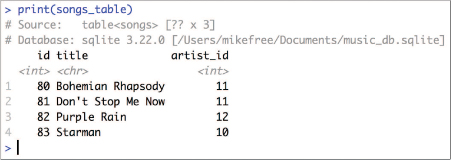
tbl, printed in RStudio.This is only a preview of the data that will be returned by the data base.
Once you have a reference to the table, you can use the same dplyr functions discussed in Chapter 11 (e.g., select(), filter()). Just use the table in place of the data frame to manipulate!
# Construct a query from the `songs_table` for songs by Queen (artist ID 11)
queen_songs_query <- songs_table %>%
  filter(artist_id == 11) %>%
  select(title)
The dbplyr package will automatically convert a sequence of dplyr functions into an equivalent SQL statement, without the need for you to write any SQL! You can see the SQL statement it is generating by using the show_query() function:
# Display the SQL syntax stored in the query `queen_songs_query`
show_query(queen_songs_query)
    # <SQL>
    # SELECT `title`
    # FROM `songs`
    # WHERE (`artist_id` = 11.0)
Importantly, using dplyr methods on a table does not return a data frame (or even a tibble). In fact, it displays just a small preview of the requested data! Actually querying the data from a database is relatively slow in comparison to accessing data in a data frame, particularly when the database is on a remote computer. Thus dbplyr uses lazy evaluation—it actually executes the query on the database only when you explicitly tell it to do so. What is shown when you print the queen_songs_query is just a subset of the data; the results will not include all of the rows returned if there are a large number of them! RStudio very subtly indicates that the data is just a preview of what has been requested—note in Figure 13.6 that the dimensions of the songs_table are unknown (i.e., table<songs> [?? X 3]). Lazy evaluation keeps you from accidentally making a large number of queries and downloading a huge amount of data as you are designing and testing your data manipulation statements (i.e., writing your select() and filter() calls).
To actually query the database and load the results into memory as a R value you can manipulate, use the collect() function. You can often add this function call as a last step in your pipe of dplyr calls.
# Execute the `queen_songs_query` request, returning the *actual data*
# from the database
queen_songs_data <- collect(queen_songs_query) # returns a tibble
This tibble is exactly like those described in earlier chapters; you can use as.data.frame() to convert it into a data frame. Thus, anytime you want to query data from a database in R, you will need to perform the following steps:
# 1. Create a connection to an RDMS, such as a SQLite database
db_connection <- dbConnect(SQLite(), dbname = "path/to/database.sqlite")

# 2. Access a specific table within your database
some_table <- tbl(db_connection, "TABLE_NAME")

# 3. Construct a query of the table using `dplyr` syntax
db_query <- some_table %>%
  filter(some_column == some_value)

# 4. Execute your query to return data from the database
results <- collect(db_query)

# 5. Disconnect from the database when you're finished
dbDisconnect(db_connection)
And with that, you have accessed and queried a database using R! You can now write R code to use the same dplyr functions for either a local data frame or a remote database, allowing you to test and then expand your data analysis.
Tip
For more information on using dbplyr, check out the introduction vignette.a
ahttps://cran.r-project.org/web/packages/dbplyr/vignettes/dbplyr.html
For practice working with databases, see the set of accompanying book exercises.10
10Database exercises: https://github.com/programming-for-data-science/chapter-13-exercises