Chapter 1. Quantum Circuits and Operations
In Qiskit, quantum programs are normally expressed by placing quantum operations on quantum circuits. Quantum circuits are represented by the QuantumCircuit class, and quantum operations are represented by subclasses of the Instruction class.
Constructing Quantum Circuits
A quantum circuit may be created by supplying an argument that indicates the number of desired quantum wires for that circuit. This is often supplied as an integer:
QuantumCircuit(2)
Optionally, the number of desired classical wires may also be specified:
QuantumCircuit(2,2)
The number of desired quantum and classical wires may also be expressed by supplying instances of QuantumRegister and ClassicalRegister as arguments to QuantumCircuit. These classes are addressed in “Using the QuantumRegister Class” and “Using the ClassicalRegister Class”.
Using the QuantumCircuit Class
The QuantumCircuit class contains a large number of methods and attributes. The purpose of many of its methods is to apply quantum operations to a quantum circuit. Most of its other methods and attributes either manipulate, or report information about, a quantum circuit.
Commonly used gates
Table 1-1 contains some commonly used single-qubit gates and code examples. Variable qc refers to an instance of QuantumCircuit that contains at least four quantum wires:
| Names | Example | Notes |
|---|---|---|
H, Hadamard |
|
Applies H gate to qubit 0. See “HGate”. |
I, Identity |
|
Applies I gate to qubit 2. See “IGate”. |
P, Phase |
|
Applies P gate with π/2 phase rotation to qubit 0. See “PhaseGate”. |
RX |
|
Applies RX gate with π/4 rotation to qubit 2. See “RXGate”. |
RY |
|
Applies RY gate with π/8 rotation to qubit 0. See “RYGate”. |
RZ |
|
Applies RZ gate with π/2 rotation to qubit 1. See “RZGate”. |
S |
|
Applies S gate to qubit 3. Equivalent to P gate with π/2 phase rotation. See “SGate”. |
S† |
|
Applies S† gate to qubit 3. Equivalent to P gate with 3π/2 phase rotation. See “SdgGate”. |
SX |
|
Applies SX (square root of X) gate to qubit 2. This is equivalent to an RX gate with a π/2 rotation. See “SXGate”. |
T |
|
Applies T gate to qubit 1. Equivalent to P gate with π/4 phase rotation. See “TGate”. |
T† |
|
Applies T† gate to qubit 1. Equivalent to P gate with 7π/4 phase rotation. See “TdgGate”. |
U |
|
Applies rotation with 3 Euler angles to qubit 1. See “UGate”. |
X, NOT |
|
Applies X gate to qubit 3. See “XGate”. |
Y |
|
Applies Y gates to qubits 0, 2 and 3. See “YGate”. |
Z |
|
Applies Z gate to qubit 2. Equivalent to P gate with π phase rotation. See “ZGate”. |
Figure 1-1 contains a nonsensical circuit with all of the single-qubit gate examples from Table 1-1
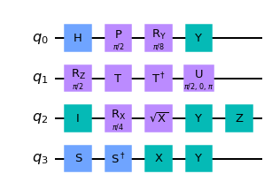
Figure 1-1. Nonsensical circuit with single-qubit gate examples
Table 1-2 contains some commonly used multi-qubit gates and code examples. Variable qc refers to an instance of QuantumCircuit that contains at least four quantum wires:
| Names | Example | Notes |
|---|---|---|
CCX, Toffoli |
|
Applies the X gate to quantum wire 2, subject to the state of the control qubits on wires 0 and 1. See “CCXGate”. |
CH |
|
Applies the H gate to quantum wire 1, subject to the state of the control qubit on wire 0. See “CHGate”. |
CP, Control-Phase |
|
Applies the Phase gate to quantum wire 1, subject to the state of the control qubit on wire 0. See “CPhaseGate”. |
CRX, Control-RX |
|
Applies the RX gate to quantum wire 3, subject to the state of the control qubit on wire 2. See “CRXGate”. |
CRY, Control-RY |
|
Applies the RY gate to quantum wire 3, subject to the state of the control qubit on wire 2. See “CRYGate”. |
CRZ |
|
Applies the RZ gate to quantum wire 1, subject to the state of the control qubit on wire 0. See “CRZGate”. |
CSwap, Fredkin |
|
Swaps the qubit states of wires 2 & 3, subject to the state of the control qubit on wire 0. See “CSwapGate”. |
CSX |
|
Applies the SX (square root of X) gate to quantum wire 1, subject to the state of the control qubit on wire 0. See “CSXGate”. |
CU |
|
Applies the U gate with an additional global phase argument to quantum wire 1, subject to the state of the control qubit on wire 0. See “CUGate”. |
CX, CNOT |
|
Applies the X gate to quantum wire 3, subject to the state of the control qubit on wire 2. See “CXGate”. |
CY, Control-Y |
|
Applies the Y gate to quantum wire 3, subject to the state of the control qubit on wire 2. See “CYGate”. |
CZ, Control-Z |
|
Applies the Z gate to quantum wire 2, subject to the state of the control qubit on wire 1. See “CYGate”. |
DCX |
|
Applies two CNOT gates whose control qubits are on wires 2 and 3. See “DCXGate”. |
iSwap |
|
Swaps the qubit states of wires 0 & 1, and changes the phase of the |
MCP, Multi-control Phase |
|
Applies the Phase gate to quantum wire 3, subject to the state of the control qubits on wires 0, 1 and 2. See “MCPhaseGate”. |
MCX, Multi-control X |
|
Applies the X gate to quantum wire 3, subject to the state of the control qubits on wires 0, 1 and 2. See “MCXGate”. |
Swap |
|
Swaps the qubit states of wires 2 & 3. See “SwapGate”. |
Figure 1-2 contains a nonsensical circuit with all of the multi-qubit gate examples from Table 1-2
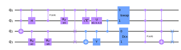
Figure 1-2. Nonsensical circuit with multi-qubit gate examples
Drawing a Quantum Circuit
The draw() method draws a quantum circuit in various formats.
Using the draw() method
Example 1-1 contains an example that uses the draw() method in the default format.
Example 1-1. Example of using the draw() method
qc=QuantumCircuit(3)qc.h(0)qc.cx(0,1)qc.cx(0,2)qc.draw()
Figure 1-3 shows the drawn circuit.

Figure 1-3. Example circuit visualization using the draw() method
Creating a Barrier
The barrier() method places a barrier on a circuit (shown in Figure 1-4), providing both visual and functional separation between gates on a quantum circuit. Gates on either side of a barrier are not candidates for being optimized together as the circuit is converted to run on quantum hardware or a simulator.
Note
The set of gates expressed using Qiskit represents an abstraction for the actual gates implemented on a given quantum computer or simulator. Qiskit transpiles the gates into those implemented on the target platform, combining gates where possible to optimize the circuit.
Using the barrier() method
The barrier() method takes as an optional argument the qubit wires on which to place a barrier. If no argument is supplied, a barrier is placed across all of the quantum wires. This method creates a Barrier instance (see “Barrier”).
Example 1-2 demonstrates using the barrier() method with and without arguments.
Example 1-2. Example of using the barrier() method
qc=QuantumCircuit(2)qc.h([0,1])qc.barrier()qc.x(0)qc.x(0)qc.s(1)qc.barrier([1])qc.s(1)
Figure 1-4 shows the resultant circuit.
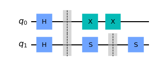
Figure 1-4. Example circuit using the barrier() method
Notice that the S gates in the circuit are separated by a barrier, and therefore not candidates to be combined into a Z gate. However the X gates may be combined by removing both of them, as they cancel each other.
Measuring a quantum circuit
The methods commonly used to measure quantum circuits are measure() and measure_all(). The former is useful when the quantum circuit contains classical wires on which to receive the result of a measurement. The latter is useful when the quantum circuit doesn’t have any classical wires. These methods create Measure instances (see “Measure”).
Using the measure() method
The measure() method takes two arguments:
-
the qubit wires to be measured
-
the classical wires on which to store the resulting bits
Here is an example of using the measure() method, as well as a drawing of the resultant circuit:
Example 1-3. Example of using the measure() method
qc=QuantumCircuit(3,3)qc.h([0,1,2])qc.measure([0,1,2],[0,1,2])qc.draw()

Figure 1-5. Example circuit using the measure() method
Notice that the measure() method appended the requested measurement operations to the circuit.
Using the measure_all() method
The measure_all() method may be called with no arguments. Here is an example of using the measure_all() method, as well as a drawing of the resultant circuit:
Example 1-4. Example of using the measure_all() method
qc=QuantumCircuit(3)qc.h([0,1,2])qc.measure_all()qc.draw()

Figure 1-6. Example circuit using the measure_all() method
Notice that the measure_all() method created three classical wires, and added a barrier to the circuit, before appending the measurement operations.
Obtaining information about a quantum circuit
Methods commonly used to obtain information about a quantum circuit include depth(), size(), and width(). These are listed in Table 1-3. Note that variable qc refers to an instance of QuantumCircuit.
| Names | Example | Notes |
|---|---|---|
|
|
Returns the depth (critical path) of a circuit if directives such as barrier were removed |
|
|
Returns the total number of gate operations in a circuit |
|
|
Return the sum of qubits wires and classical wires in a circuit |
Attributes commonly used to obtain information about a quantum circuit include clbits, data, global_phase, num_clbits, num_qubits, and qubits. These are listed in Table 1-4. Note that variable qc refers to an instance of QuantumCircuit.
| Names | Example | Notes |
|---|---|---|
|
|
Obtains the list of classical bits in the order that the registers were added |
|
|
Obtains a list of the operations (e.g. gates, barriers, and measurement operations) in the circuit |
|
|
Obtains the global phase of the circuit in radians |
|
|
Obtains the number of classical wires in the circuit |
|
|
Obtains the number of quantum wires in the circuit |
|
|
Obtains the list of quantum bits in the order that the registers were added |
Manipulating a quantum circuit
Methods commonly used to manipulate quantum circuits include append(), bind_parameters(), compose(), copy(), decompose(), from_qasm_file(), from_qasm_str(), initialize(), reset(), qasm(), to_gate(), and to_instruction().
Using the append() method
The append() method appends an instruction or gate to the end of the circuit on specified wires, modifying the circuit in place. Example 1-5 contains an example of using the append() method, and Figure 1-7 shows a drawing of the resultant circuit.
Example 1-5. Example of using the append() method
qc=QuantumCircuit(2)qc.h(1)cx_gate=CXGate()qc.append(cx_gate,[1,0])qc.draw()
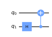
Figure 1-7. Example circuit resulting from the append() method
Note
The CXGate class (see “CXGate”) used in the example is one of the gates defined in the qiskit.circuit.library package.
Using the bind_parameters() method
The bind_parameters() method binds parameters (see “Creating a Parameter Instance”) to a quantum circuit. Example 1-6 contains an example of creating a circuit in which there are three parameterized phase gates. Figure 1-8 shows a drawing of the circuit.
Example 1-6. Creating a parameterized circuit
theta1=Parameter('θ1')theta2=Parameter('θ2')theta3=Parameter('θ3')qc=QuantumCircuit(3)qc.h([0,1,2])qc.p(theta1,0)qc.p(theta2,1)qc.p(theta3,2)qc.draw()

Figure 1-8. Example parameterized circuit
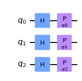
To bind the parameter values to a new circuit, we’ll pass a dictionary that contains the parameter references and desired values to the bind_parameters() method. Example 1-7 shows this technique, and Figure 1-9 shows the bound circuit in which the phase gate parameters are replaced with the supplied values.
Example 1-7. Binding parameter values to a new circuit
b_qc=qc.bind_parameters({theta1:math.pi/8,theta2:math.pi/4,theta3:math.pi/2})b_qc.draw()

Figure 1-9. Example of bound circuit with the supplied phase gate rotation values
Using the compose() method
The compose() method returns a new circuit composed of the original and another circuit. Example 1-8 contains an example of using the compose() method, and Figure 1-10 shows a drawing of the resultant circuit.
Example 1-8. Example of using the compose() method
qc=QuantumCircuit(2,2)qc.h(0)another_qc=QuantumCircuit(2,2)another_qc.cx(0,1)bell_qc=qc.compose(another_qc)bell_qc.draw()
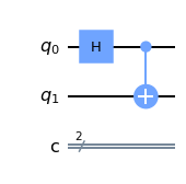
Figure 1-10. Example circuit resulting from the compose() method
Note that a circuit passed into the compose() method is allowed to have fewer quantum or classical wires than the original circuit.
Using the copy() method
The copy() method returns a copy of the original circuit. Example 1-9 contains an example of using the copy() method.
Example 1-9. Example of using the copy() method
qc=QuantumCircuit(3)qc.h([0,1,2])new_qc=qc.copy()
Using the decompose() method
The decompose() method returns a new circuit after having decomposed the original circuit one level. Example 1-10 contains an example of using the decompose() method. Figure 1-11 shows a drawing of the resultant circuit in which S, H, and X gates are decomposed into the more fundamental U gate operations. See “UGate”.
Example 1-10. Example of using the decompose() method
qc=QuantumCircuit(2)qc.h(0)qc.s(0)qc.x(1)decomposed_qc=qc.decompose()decomposed_qc.draw()
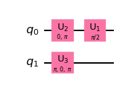
Figure 1-11. Example circuit resulting from the decompose() method
Using the from_qasm_file() method
The from_qasm_file() method returns a new circuit from a file that contains a quantum assembly-language (OpenQASM) program. Example 1-11 contains an example of using the from_qasm_file() method.
Example 1-11. Example of using the from_qasm_file() method
new_qc=QuantumCircuit.from_qasm_file("file.qasm")
Using the from_qasm_str() method
The from_qasm_str() method returns a new circuit from a string that contains an OpenQASM program. Example 1-12 contains an example of using the from_qasm_str() method, and Figure 1-12 shows a drawing of the resultant circuit.
Example 1-12. Example of using the from_qasm_str() method
qasm_str="""OPENQASM 2.0;include "qelib1.inc";qreg q[2];creg c[2];h q[0];cx q[0],q[1];measure q[0] -> c[0];measure q[1] -> c[1];"""new_qc=QuantumCircuit.from_qasm_str(qasm_str)new_qc.draw()
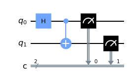
Figure 1-12. Example circuit resulting from the from_qasm_str() method
Using the initialize() method
The initialize() method initializes qubits of a quantum circuit to a given state. Example 1-13 contains an example of using the initialize() method, and Figure 1-13 shows a drawing of the resultant circuit. In this example, the circuit is initialized to the state ![]() .
.
Example 1-13. Example of using the initialize() method
qc=QuantumCircuit(2)qc.initialize([0,0,0,1])qc.draw()
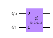
Figure 1-13. Example circuit resulting from the initialize() method
Using the reset() method
The reset() method resets a qubit in a quantum circuit to the ![]() state. Example 1-14 contains an example of using the
state. Example 1-14 contains an example of using the reset() method, and Figure 1-14 shows a drawing of the resultant circuit. Note that the qubit state is ![]() before the reset operation. This method creates a
before the reset operation. This method creates a Reset instance (see “Reset”).
Example 1-14. Example of using the reset() method
qc=QuantumCircuit(1)qc.x(0)qc.reset(0)qc.draw()

Figure 1-14. Example circuit resulting from the using the reset() method
Using the qasm() method
The qasm() method returns an OpenQASM program that represents the quantum circuit. Example 1-15 contains an example of using the qasm() method, and Example 1-16 shows the resultant OpenQASM program.
Example 1-15. Example of using the qasm() method
qc=QuantumCircuit(2,2)qc.h(0)qc.cx(0,1)qasm_str=qc.qasm()(qasm_str)
Example 1-16. OpenQASM program resulting from the using the qasm() method
OPENQASM2.0;include"qelib1.inc";qregq[2];cregc[2];hq[0];cxq[0],q[1];
Using the to_gate() method
The to_gate() method creates a custom gate (see “The Gate Class”) from a quantum circuit. Example 1-17 contains an example of creating a circuit that will be converted to a gate, and Figure 1-15 shows a drawing of the circuit.
Note
A gate represents a unitary operation. To create a custom operation that isn’t unitary, use the to_instruction() method shown in “Using the to_instruction() method”.
Example 1-17. Creating a circuit that will be converted to a gate
anti_cnot_qc=QuantumCircuit(2)anti_cnot_qc.x(0)anti_cnot_qc.cx(0,1)anti_cnot_qc.x(0)anti_cnot_qc.draw()

Figure 1-15. Example circuit that will be converted to a gate
This custom gate will implement an anti-control NOT gate in which the X gate is applied only when the control qubit is ![]() . Example 1-18 creates a circuit that uses this custom gate, and Figure 1-16 shows a decomposed drawing of this circuit.
. Example 1-18 creates a circuit that uses this custom gate, and Figure 1-16 shows a decomposed drawing of this circuit.
Example 1-18. Example of using a gate created by the to_gate() method
anti_cnot_gate=anti_cnot_qc.to_gate()qc=QuantumCircuit(3)qc.x([0,1,2])qc.append(anti_cnot_gate,[0,2])qc.decompose().draw()

Figure 1-16. Decomposed circuit that uses a gate created by the to_gate() method
Using the to_instruction() method
The to_instruction() method creates a custom instruction (see “The Instruction Class”) from a quantum circuit. Example 1-19 contains an example of creating a circuit that will be converted to an instruction, and Figure 1-17 shows a drawing of the circuit.
Note
An instruction represents an operation that isn’t necessarily unitary. To create a custom operation that is unitary, use the to_gate() method shown in “Using the to_gate() method”.
Example 1-19. Creating a circuit that will be converted to an instruction
reset_one_qc=QuantumCircuit(1)reset_one_qc.reset(0)reset_one_qc.x(0)reset_one_qc.draw()

Figure 1-17. Example circuit that will be converted to an instruction
This custom instruction will reset a qubit and apply an X gate, in effect resetting the qubit to state ![]() . Example 1-20 creates a circuit that uses this custom instruction, and Figure 1-18 shows a decomposed drawing of this circuit.
. Example 1-20 creates a circuit that uses this custom instruction, and Figure 1-18 shows a decomposed drawing of this circuit.
Example 1-20. Example of using an instruction created by the to_instruction() method
reset_one_inst=reset_one_qc.to_instruction()qc=QuantumCircuit(2)qc.h([0,1])qc.reset(0)qc.append(reset_one_inst,[1])qc.decompose().draw()

Figure 1-18. Circuit that uses an instruction created by the to_instruction() method
Saving state when running a circuit on AerSimulator
When running a circuit on an AerSimulator backend (see [Link to Come]), simulator state may be saved in the circuit instance by using the QuantumCircuit methods in Table 1-5.
| Method name | Description |
|---|---|
|
Saves the simulator state as appropriate for the simulation method |
|
Saves the simulator state as a density matrix |
|
Saves the simulator state as a matrix product state tensor |
|
Saves the simulator state as a Clifford stabilizer |
|
Saves the simulator state as a statevector |
|
Saves the simulator state as a superoperator matrix of the run circuit |
|
Saves the simulator state as a unitary matrix of the run circuit |
Using the QuantumRegister Class
It is sometimes useful to treat groups of quantum or classical wires as a unit. For example, the control qubits of the CNOT gates in the quantum circuit expressed in Example 1-21 and Figure 1-19 expect three qubits in equal superpositions. The additional quantum wire in the circuit is used as a scratch area whose output is disregarded.
Example 1-21. Example of using QuantumRegister and ClassicalRegister classes
qr=QuantumRegister(3,'q')scratch=QuantumRegister(1,'scratch')cr=ClassicalRegister(3,'c')qc=QuantumCircuit(qr,scratch,cr)qc.h(qr)qc.x(scratch)qc.h(scratch)qc.cx(qr[0],scratch)qc.cx(qr[2],scratch)qc.barrier(qr)qc.h(qr)qc.measure(qr,cr)qc.draw()
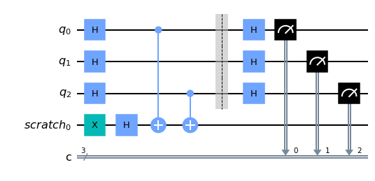
Figure 1-19. Example circuit using the QuantumRegister and ClassicalRegister classes
By defining a QuantumRegister consisting of three qubits, methods such as h(), barrier(), and measure() may be applied to all three wires by passing a QuantumRegister reference. Similarly, defining a ClassicalRegister (see “Using the ClassicalRegister Class”) consisting of three bits enables the measure() method to specify all three classical wires by passing a ClassicalRegister reference. Additionally, the names supplied to the QuantumRegister and ClassicalRegister constructors are displayed on the circuit drawing.
Some QuantumRegister attributes
Commonly used QuantumRegister attributes include name, and size. These are listed in Table 1-6. Note that variable qr refers to an instance of QuantumRegister.
| Names | Example | Notes |
|---|---|---|
|
|
Obtains the name the quantum register |
|
|
Obtains the number of qubit wires in the quantum register |
Using the ClassicalRegister Class
Please refer to “Using the QuantumRegister Class” for also motivating use of the ClassicalRegister class.
Some ClassicalRegister attributes
Commonly used ClassicalRegister attributes include name, and size. These are listed in Table 1-7. Note that variable cr refers to an instance of ClassicalRegister.
| Names | Example | Notes |
|---|---|---|
|
|
Obtains the name the classical register |
|
|
Obtains the number of bit wires in the classical register |
Instructions and Gates
In Qiskit, all operations that may be applied to a quantum circuit are derived from the Instruction class (see “The Instruction Class”). Unitary operations are derived from the Gate class (see “The Gate Class”), which is a subclass of Instruction. Controlled-unitary operations are derived from the ControlledGate class (see “The ControlledGate Class”), which is a subclass of Gate. These classes may be used to define new instructions, unitary gates, and controlled-unitary gates, respectively.
The Instruction Class
The non-unitary operations in Qiskit (such as Measure, and Reset) are direct subclasses of Instruction. Although it is possible to define your own custom instructions by subclassing Instruction, another way is to use the to_instruction() method of the QuantumCircuit class (see an example of this in “Using the to_instruction() method”).
Methods in the Instruction class include copy(), repeat(), and reverse_ops(). These are listed in Table 1-8. Note that variable inst refers to an instance of Instruction.
| Names | Example | Notes |
|---|---|---|
|
|
Returns a copy of the instruction, giving the supplied name to the copy |
|
|
Returns an instruction with this instruction repeated a given number of times |
|
|
Returns an instruction with its operations in reverse order |
Commonly used attributes in the Instruction class include definition, and params. These are listed in Table 1-9. Note that variable inst refers to an instance of Instruction.
| Names | Example | Notes |
|---|---|---|
|
|
Returns the definition in terms of basic gates |
|
|
Obtains the parameters to the instruction |
The Gate Class
The unitary operations in Qiskit (such as HGate, and XGate) are subclasses of Gate. Although it is possible to define your own custom gates by subclassing Gate, another way is to use the to_gate() method of the QuantumCircuit class (see an example of this in “Using the to_gate() method”).
Commonly used methods in the Gate class include the Instruction methods listed in Table 1-8 as well as control(), inverse(), power(), and to_matrix(). These are all listed in Table 1-10. Note that variable gate refers to an instance of Gate.
| Names | Example | Notes |
|---|---|---|
|
|
Given a number of control qubits, returns a controlled version of the gate |
|
|
Returns a copy of the gate, giving the supplied name to the copy |
|
|
Returns the inverse of the gate |
|
|
Returns the gate raised to a given power |
|
|
Returns a gate with this gate repeated a given number of times |
|
|
Returns a gate with its operations in reverse order |
|
|
Returns an array for the gate’s unitary matrix |
Commonly used attributes in the Gate class include the Instruction attributes listed in Table 1-9 as well as label. These are all listed in Table 1-11. Note that variable gate refers to an instance of Gate.
| Names | Example | Notes |
|---|---|---|
|
|
Returns the definition in terms of basic gates |
|
|
Obtains the label for the instruction |
|
|
Obtains the parameters to the instruction |
The ControlledGate Class
The controlled-unitary operations in Qiskit (such as CZGate, and CCXGate) are subclasses of ControlledGate.
Commonly used methods in the ControlledGate class are the Gate methods listed in Table 1-10
Commonly used attributes in the ControlledGate class include the Gate attributes listed in Table 1-11 as well as num_ctrl_qubits, and ctrl_state.
Using the num_ctrl_qubits attribute
The num_ctrl_qubits attribute holds an integer that represents the number of control qubits in a ControlledGate. Example 1-22 contains an example of using the num_ctrl_qubits attribute of a Toffoli gate, whose printed output would be 2.
Example 1-22. Example of using the num_ctrl_qubits attribute
toffoli=CCXGate()(toffoli.num_ctrl_qubits)
Using the ctrl_state() method
A ControlledGate may have one or more control qubits, each of which may actually be either control or anti-control qubits (see anti-control example in “Using the to_gate() method”). The ctrl_state attribute holds an integer whose binary value represents which qubits are control qubits, and which are anti-control qubits. Specifically, the binary digit 1 represents a control qubit, and the binary digit 0 represents an anti-control qubit. The ctrl_state attribute supports both accessing and modifying its value. Example 1-23 contains an example of using the ctrl_state attribute in which the binary value 10 causes the topmost control qubit to be an anti-control qubit.
Example 1-23. Example of using the ctrl_state attribute
toffoli=CCXGate()toffoli.ctrl_state=2toffoli.definition.draw()
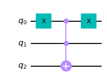
Figure 1-20. Toffoli gate with a control qubit and an anti-control qubit
Defining a custom controlled gate
Although it is possible to define your own custom controlled gates by subclassing ControlledGate, another way is to follow these two steps:
-
Create a custom gate with the
to_gate()method of theQuantumCircuitclass (see an example of this in “Using the to_gate() method”) -
Add control qubits to your custom gate with the
control()method shown in Table 1-10
We’ll follow those two steps to define a custom controlled gate that applies a π/16 phase rotation when both of its control qubits are ![]() . First, Example 1-24 defines a circuit that contains a π/16 P gate and converts it to a custom gate, with Figure 1-21 showing a drawing of the custom gate.
. First, Example 1-24 defines a circuit that contains a π/16 P gate and converts it to a custom gate, with Figure 1-21 showing a drawing of the custom gate.
Example 1-24. Creating a custom π/16 phase gate
p16_qc=QuantumCircuit(1)p16_qc.p(math.pi/16,0)p16_gate=p16_qc.to_gate()p16_gate.definition.draw()
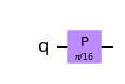
Figure 1-21. Custom π/16 phase gate drawing
Second, Example 1-25 uses the control() method to create a ControlledGate from our custom gate, and Figure 1-22 shows a drawing of the custom controlled gate.
Example 1-25. Example of using the control() method to add control qubits to a gate
ctrl_p16=p16_gate.control(2)ctrl_p16.definition.draw()

Figure 1-22. Custom controlled π/16 phase gate drawing
We’ll leverage the append() method (see “Using the append() method”) in Example 1-26 to use our custom controlled gate in a quantum circuit. Figure 1-22 shows a drawing of the circuit.
Example 1-26. Example of using a gate created by the to_gate() method
qc=QuantumCircuit(4)qc.h([0,1,2,3])qc.append(ctrl_p16,[0,1,3])qc.draw()

Figure 1-23. Decomposed circuit that uses the custom controlled gate
Parameterized Quantum Circuits
It is sometimes useful to create a quantum circuit in which values may be supplied at runtime. This capability is available in Qiskit using parameterized circuits, implemented in part by the Parameter, and ParameterVector classes.
Creating a Parameter Instance
The Parameter class is used to represent a parameter in a quantum circuit. See “Using the bind_parameters() method” for an example of defining and using a parameterized circuit. As shown in that example, a parameter may be created by supplying a unicode string to its constructor as follows:
theta1 = Parameter("θ1")
The Parameter object reference named theta1 may subsequently be used in the bind_parameters(), or alternatively the assign_parameters(), method of the QuantumCircuit class.
Using the ParameterVector Class
The ParameterVector class may be leveraged to create and use parameters as a collection instead of individual variables. Example 1-27 contains an example of creating a circuit in which there are three parameterized phase gates. Figure 1-24 shows a drawing of the circuit.
Example 1-27. Leveraging ParameterVector to create a parameterized circuit
theta=ParameterVector('θ',3)qc=QuantumCircuit(3)qc.h([0,1,2])qc.p(theta[0],0)qc.p(theta[1],1)qc.p(theta[2],2)qc.draw()

Figure 1-24. Example parameterized circuit leveraging ParameterVector
To bind the parameter values to a new circuit, we’ll pass a dictionary that contains the ParameterVector reference and desired list of values to the bind_parameters() method. Example 1-28 shows this technique, and Figure 1-25 shows the bound circuit in which the phase gate parameters are replaced with the supplied values.
Example 1-28. Binding parameter values to a new circuit
b_qc=qc.bind_parameters({theta:[math.pi/8,math.pi/4,math.pi/2]})b_qc.draw()