
Chapter 1
Introduction and how to use this book
Abstract
The primary purpose of this book is to provide a statistical resource for those who measure the behavior and attitudes of people as they interact with interfaces. Our focus is on methods applicable to practical user research, based on our experience, investigations, and reviews of the latest statistical literature. As an aid to the persistent problem of remembering what method to use under what circumstances, this chapter contains four decision maps to guide researchers to the appropriate method and its chapter in this book.
Keywords
user experience
user research
summarizing data
margin of error
confidence interval
statistical test
comparison of groups
comparison with a benchmark
discrete-binary data
continuous data
decision map
Introduction
The last thing many designers and researchers in the field of user experience think of is statistics. In fact, we know many practitioners who find the field appealing because it largely avoids those impersonal numbers. The thinking goes that if usability and design are qualitative activities, it’s safe to skip the formulas and numbers.
Although design and several usability activities are certainly qualitative, the impact of good and bad designs can easily be quantified in conversions, completion rates, completion times, perceived satisfaction, recommendations, and sales. Increasingly, usability practitioners and user researchers are expected to quantify the benefits of their efforts. If they don’t, someone else will—unfortunately that someone else might not use the right metrics or methods.
The organization of this book
This book is intended for those who measure the behavior and attitudes of people as they interact with interfaces. This book is not about abstract mathematical theories for which you may someday find a partial use. Instead, this book is about working backwards from the most common questions and problems you’ll encounter as you conduct, analyze, and report on user research projects. In general, these activities fall into four areas:
1. Summarizing data and computing margins of error (Chapter 3)
2. Determining if there is a statistically significant difference, either in comparison to a benchmark (Chapter 4) or between groups (Chapters 5 and 10)
4. Investigating relationships among variables (Chapter 10).
We also provide:
• Background chapters with an overview of common ways to quantify user research (Chapter 2) and a quick introduction/review of many fundamental statistical concepts (Appendix)
• A comprehensive discussion of standardized usability questionnaires (Chapter 8)
• A discussion of enduring statistical controversies of which user researchers should be aware and able to articulate in defense of their analyses (Chapter 9)
• A wrap-up chapter with pointers to more information on statistics for user research (Chapter 11)
Each chapter ends with a list of key points and references. Most chapters also include a set of problems and answers to those problems so you can check your understanding of the content.
How to use this book
Despite there being a significant proportion of user research practitioners with advanced degrees, about 7% have PhDs (UXPA, 2014), for most people in the social sciences statistics is the only quantitative course they have to take. For many, statistics is a subject they know they should understand, but it often brings back bad memories of high-school math, poor teachers, and an abstract and difficult topic.
While we’d like to take all the pain out of learning and using statistics, there are still formulas, math, and some abstract concepts that we just can’t avoid. Some people want to see how the statistics work, and for them we provide the math. If you’re not terribly interested in the computational mechanics, then you can skip over the formulas and focus more on how to apply the procedures.
Readers who are familiar with many statistical procedures and formulas may find that some of the formulas we use differ from those taught in college statistics courses. Part of this is from recent advances in statistics (especially for dealing with binary data). Another part is due to our selecting the best procedures for practical user research, focusing on procedures that work well for the types of data and sample sizes you’ll likely encounter.
Based on teaching many courses at industry conferences and at companies, we know the statistics background of the readers of this book will vary substantially. Some of you may have never taken a statistics course whereas others probably took several in graduate school. As much as possible, we’ve incorporated relevant discussions around the concepts as they appear in each chapter with plenty of examples using actual data from real user research studies.
In our experience, one of the hardest things to remember in applying statistics is what statistical test to perform when. To help with this problem, we’ve provided the following decision maps (Figs. 1.1–1.4) to help you get to the right statistical test and the sections of the book that discuss it.

Figure 1.1 Decision map for analyses of continuous data

Figure 1.2 Decision map for analysis of discrete-binary data

Figure 1.3 Decision map for sample sizes when comparing data
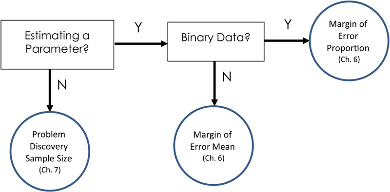
Figure 1.4 Decision map for sample sizes for estimating precision or detection
What test should I use?
The first decision point comes from the type of data you have. See the Appendix for a discussion of the distinction between discrete and continuous data. In general, for deciding which test to use, you need to know if your data are discrete-binary (e.g., pass/fail data coded as 1s and 0s) or more continuous (e.g., task times or rating scale data).
The next major decision is whether you’re comparing data or just getting an estimate of precision. To get an estimate of precision you compute a confidence interval around your sample metrics (e.g., what is the margin of error around a completion rate of 70%—see Chapter 3). By comparing data we mean comparing data from two or more groups (e.g., task completion times for Product A and B—see Chapter 5) or comparing your data to a benchmark (e.g., is the completion rate for Product A significantly above 70%?—see Chapter 4).
If you’re comparing data, the next decision is whether the groups of data come from the same or different users. Continuing on that path, the final decision depends on whether there are two groups to compare or more than two groups.
To find the appropriate section in each chapter for the methods depicted in Figures 1.1 and 1.2, consult Tables 1.1 and 1.2. Note that methods discussed in Chapter 11 are outside the scope of this book, and receive just a brief description in their sections.
Table 1.1
Chapter Sections for Methods Depicted in Fig. 1.1
| Method | Chapter: Section |
| One-Sample t (Log) | 4: Comparing a Task Time to a Benchmark |
| One-Sample t | 4: Comparing a Satisfaction Score to a Benchmark |
| Confidence Interval around Median | 3: Confidence Interval around a Median |
| t (Log) Confidence Interval | 3: Confidence Interval for Task-Time Data |
| t Confidence Interval | 3: Confidence Interval for Rating Scales and Other Continuous Data |
| Paired t | 5: Within-Subjects Comparison (Paired t-Test) |
| ANOVA or Multiple Paired t | 5: Within-Subjects Comparison (Paired t-Test) |
| 9: What If You Need To Run More than One Test? | |
| 11: Getting More Information: Analysis of Variance | |
| Two-Sample t | 5: Between-Subjects Comparison (Two-Sample t-Test) |
| ANOVA or Multiple Two-Sample t | 5: Between-Subjects Comparison (Two-Sample t-Test) |
| 9: What If You Need To Run More than One Test? | |
| 10: Analysis of Variance | |
| Correlation | 10: Correlation |
| Regression Analysis | 10: Regression |
Table 1.2
Chapter Sections for Methods Depicted in Fig. 1.2
| Method | Chapter: Section |
| One-Sample Z-Test | 4: Comparing a Completion Rate to a Benchmark—Large Sample Test |
| One-Sample Binomial | 4: Comparing a Completion Rate to a Benchmark—Small Sample Test |
| Adjusted Wald Confidence Interval | 3: Adjusted-Wald: Add Two Successes and Two Failures |
| McNemar Exact Test | 5: McNemar Exact Test |
| Adjusted Wald Confidence Interval for Difference in Matched Proportions | 5: Confidence Interval around the Difference for Matched Pairs |
| N−1 Two Proportion Test and Fisher Exact Test | 5: N−1 Two Proportion Test; Fisher Exact Test |
| Adjusted Wald Difference in Proportion | 5: Confidence for the Difference between Proportions |
| Correlation | 10: Correlation—Computing the Phi Correlation |
| Chi Square | 11: Getting More Information—Analysis of Many-Way Contingency Tables |
For example, let’s say you wanted to know which statistical test to use if you are comparing completion rates on an older version of a product and a new version where a different set of people participated in each test.
1. Because completion rates are discrete-binary data (1 = Pass and 0 = Fail), we should use the decision map in Fig. 1.2.
2. At the first box “Comparing or Correlating Data” select “Y” because we’re planning to compare data (rather than exploring relationships with correlation or regression).
3. At the next box “Comparing Data?” select “Y” because we are comparing a set of data from an older product with a set of data from a new product.
4. This takes us to the “Different Users in Each Group” box—we have different users in each group, so we select “Y.”
5. Now we’re at the “Three or More Groups” box—we have only two groups of users (before and after) so we select “N.”
What sample size do I need?
Often the first collision a user researcher has with statistics is in planning sample sizes. Although there are many “rules of thumb” on how many users you should test or how many customer responses you need to achieve your goals, there really are precise ways of estimating the answer. The first step is to identify the type of test for which you’re collecting data. In general, there are three ways of determining your sample size:
1. Estimating a parameter with a specified precision (e.g., if your goal is to estimate completion rates with a margin of error of no more than 5%, or completion times with a margin of error of no more than 15 s)
2. Comparing two or more groups or comparing one group to a benchmark
3. Problem discovery, specifically, the number of users you need in a usability test to find a specified percentage of usability problems with a specified probability of occurrence.
To find the appropriate section in each chapter for the methods depicted in Figs. 1.3 and 1.4, consult Table 1.3.
Table 1.3
Chapter Sections for Methods Depicted in Figs. 1.3 and 1.4
| Method | Chapter: Section |
| Two Proportions | 6: Sample Size estimation for Chi-Squared Tests (Independent Proportions) |
| Two Means | 6: Comparing Values—Example 6 |
| Paired Proportions | 6: Sample Size Estimation for McNemar Exact Tests (Matched Proportions) |
| Paired Means | 6: Comparing Values—Example 5 |
| Proportion to Criterion | 6: Sample Size for Comparison with a Benchmark Proportion |
| Mean to Criterion | 6: Comparing Values—Example 4 |
| Margin of Error Proportion | 6: Sample Size Estimation for Binomial Confidence Intervals |
| Margin of Error Mean | 6: Estimating Values—Examples 1–3 |
| Problem Discovery Sample Size | 7: Using a Probabilistic Model of Problem Discovery to Estimate Sample Sizes for Formative User Research |
| Sample Size for Correlation | 10: Sample Size Estimation for r |
| Sample Size for Linear Regression | 10: Sample Size Estimation for Linear Regression |
For example, let’s say you wanted to compute the appropriate sample size if the same users will rate the usability of two products using a standardized questionnaire that provides a mean score.
1. Because the goal is to compare data, start with the sample size decision map in Fig. 1.3.
2. At the “Comparing or Correlating Data?” box, select Y because you’re planning to compare data (rather than exploring their relationship with correlation or regression).
3. At the “Comparing?” box, select “Y” because there will be two groups of data, one for each product.
4. At the “Different Users in each Group?” box, select “N” because each group will have the same users.
5. Because rating-scale data are not binary, select “N” at the “Binary Data?” box.
6. Stop at the “Paired Means” procedure (Chapter 6).
You don’t have to do the computations by hand
We’ve provided sufficient detail in the formulas and examples that you should be able to do all computations in Microsoft Excel. If you have an existing statistical package like SPSS, Minitab, or SAS, you may find some of the results will differ (like confidence intervals and sample size computations) or they don’t include some of the statistical tests we recommend, so be sure to check the notes associated with the procedures.
We’ve created an Excel calculator that performs all the computations covered in this book. It includes both standard statistical output (p-values and confidence intervals) and some more user-friendly output that, for example, reminds you how to interpret that ubiquitous p-value and which you can paste right into reports. It is available for purchase online at: www.measuringu.com/products/expandedStats. For detailed information on how to use the Excel calculator (or a custom set of functions written in the R statistical programming language) to solve the over 100 quantitative examples and exercises that appear in this book, see Lewis and Sauro (2016).
Key points
• The primary purpose of this book is to provide a statistical resource for those who measure the behavior and attitudes of people as they interact with interfaces.
• Our focus is on methods applicable to practical user research, based on our experience, investigations, and reviews of the latest statistical literature.
• As an aid to the persistent problem of remembering what method to use under what circumstances, this chapter contains four decision maps to guide researchers to the appropriate method and its chapter in this book.
Chapter review questions
1. Suppose you need to analyze a sample of task-time data against a specified benchmark. For example, you want to know if the average task time is less than two min. What procedure should you use?
2. Suppose you have some conversion-rate data and you just want to understand how precise the estimate is. For example, in examining the server log data you see 10,000 page views and 55 clicks on a registration button. What procedure should you use?
3. Suppose you’re planning to conduct a study in which the primary goal is to compare task completion times for two products, with two independent groups of participants providing the times. Which sample size estimation method should you use?
4. Suppose you’re planning to run a formative usability study—one where you’re going to watch people use the product you’re developing and see what problems they encounter. Which sample size estimation method should you use?
Answers to chapter review questions
1. Task-time data are continuous (not binary-discrete), so start with the decision map in Fig. 1.1. Because you’re testing against a benchmark rather than comparing or correlating groups of data, follow the N path from “Comparing or Correlating Data?” At “Testing Against a Benchmark?”, select the Y path. Finally, at “Task Time?”, take the Y path, which leads you to “One-Sample t (Log).” As shown in Table 1.1, you’ll find that method discussed in Chapter 4 in the section “Comparing a Task Time to a Benchmark” section on p. 52.
2. Conversion-rate data are binary-discrete, so start with the decision map in Fig. 1.2. You’re just estimating the rate rather than comparing a set of rates, so at “Comparing or Correlating Data,” take the N path. At “Testing Against a Benchmark?”, also take the N path. This leads you to “Adjusted Wald Confidence Interval,” which, according to Table 1.2, is discussed in Chapter 3 in the section “Adjusted-Wald: Add Two Successes and Two Failures” section on p. 22.
3. Because you’re planning a comparison of two independent sets of task times, start with the decision map in Fig. 1.3. At “Comparing or Correlating Data?”, select the Y path. At “Comparing”, select the Y path. At Different Users in each Group?”, select the Y path. At “Binary Data?”, select the N path. This takes you to “Two Means,” which, according to Table 1.3, is discussed in Chapter 6 in the section “Comparing Values—Example 6.” See Example 6 on p. 114.
4. For this type of problem discovery evaluation, you’re not planning any type of comparison, so start with the decision map in Fig. 1.4. You’re not planning to estimate any parameters such as task times or problem occurrence rates, so at “Estimating a Parameter?”, take the N path. This leads you to “Problem Discovery Sample Size” which, according to Table 1.3, is discussed in Chapter 7 in the section “Using a Probabilistic Model of Problem Discovery to Estimate Sample Sizes for Formative User Research” section on p. 143.
..................Content has been hidden....................
You can't read the all page of ebook, please click here login for view all page.