
Chapter 7
What sample sizes do we need? Part 2: formative studies
Abstract
The purpose of formative user research is to discover and enumerate the events of interest in the study (e.g., the problems that participants experience during a formative usability study). The statistical methods used to estimate sample sizes for formative research draw upon techniques not routinely taught in introductory statistics classes. This chapter covers techniques based on the binomial probability model and discusses issues associated with violation of the assumptions of the binomial model when averaging probabilities across a set of problems or participants while maintaining a focus on practical aspects of iterative design.
Keywords
sample size estimation
formative user research
problem discovery
binomial model
binomial probability formula
adjustment of estimates from small samples
deflation adjustment
Good-Turing discounting
undiscovered problems
discovery goal
Magic Number 5
beta-binomial model
logit-normal binomial model
capture-recapture model
heterogeneity
robustness
Introduction
Sample size estimation for summative usability studies (the topic of the previous chapter) draws upon techniques that are either the same as or closely related to methods taught in introductory statistics classes at the university level, with application to any user research in which the goal is to obtain measurements. In contrast to the measurements taken during summative user research, the goal of a formative usability study is to discover and enumerate the problems that users have when performing tasks with a product. It is possible, though, using methods not routinely taught in introductory statistics classes, to statistically model the discovery process and to use that model to inform sample size estimation for formative usability studies. These statistical methods for modeling the discovery of problems also have applicability for other types of user research, such as the discovery of requirements or interview themes (Guest et al., 2006).
Using a probabilistic model of problem discovery to estimate sample sizes for formative user research
The famous equation P(x ≥ 1) = 1 – (1 – p)n
The most commonly used formula to model the discovery of usability problems as a function of sample size is:
In this formula, p is the probability of an event (e.g., the probability of tossing a coin and getting heads), n is the number of opportunities for the event to occur (e.g., the number of coin tosses), and P(x ≥ 1) is the probability of the event occurring at least once in n tries.
For example, the probability of having heads come up at least once in five coin tosses (where x is the number of heads) is:
Even though the probability of heads is only 0.5, by the time you toss a coin five times you’re almost certain to have seen at least one of the tosses come up heads—in fact, out of a series of tosses of five coins, you should see at least one head about 96.9% of the time. Fig. 7.1 shows how the value of 1 – (1 – p)n changes as a function of sample size and value of p.

Figure 7.1 Probability of Discovery as a Function of n and p.
The probability of at least one equals one minus the probability of none
A lesson from James V. Bradley—from the files of Jim Lewis
There are several ways to derive 1 – (1 – p)n. For example, Nielsen and Landauer (1993) derived it from a Poisson probability process. I first encountered it in college in a statistics class I had with James V. Bradley in the late 1970s at New Mexico State University.
Dr Bradley was an interesting professor, the author of numerous statistical papers and two books: Probability; Decision; Statistics and Distribution-Free Statistical Tests. He would leave the campus by 4:00 pm every afternoon to get to his trailer in the desert because if he didn’t, he told me his neighbors would “steal everything that wasn’t nailed down.” He would teach t-tests, but would not teach analysis of variance because he didn’t believe psychological data ever met its assumptions (a view not held by the authors of this book). I had to go to the College of Agriculture’s stats classes to learn about ANOVA (see Chapter 10 for an introduction to ANOVA).
Despite these (and other) eccentricities, he was a remarkable and gifted teacher. When we were studying the binomial probability formula, one of the problems he posed to us was to figure out the probability of occurrence of at least one event of probability p given n trials. To work this out, you need to start with the binomial probability formula (Bradley, 1976), where P(x) is the probability that an event with probability p will happen x times in n trials.

The trick to solving Bradley’s problem is the realization that the probability of an event happening at least once is one minus the probability that it won’t happen at all (in other words 1 minus P(x = 0), which leads to:

Because the value of 0! is 1 and any number taken to the 0th power also equals 1, we get:

So, starting from the binomial probability formula and solving for the probability of an event occurring at least once, we derive 1 − (1 − p)n. I first applied this as a model of problem discovery to estimate sample size requirements for formative usability studies in the early 1980s (Lewis, 1982), and have always been grateful to Dr Bradley for giving us that problem to solve.
Deriving a sample size estimation equation from 1 – (1 – p)n
To convert P(x ≥ 1) = 1 – (1 – p)n to a sample-size formula, we need to solve for n. Because n is an exponent, it’s necessary to take logs, which leads to:

For these equations, we used natural logarithms (ln) to avoid having to specify the base, which simplifies the formulas. Excel provides functions for both the natural logarithm, ln, and for logarithms of specified base, log. When working with logarithms in Excel, use whichever function you prefer.
To use this equation to compute n, we need to have values for p and P(x ≥ 1). The most practical approach is to set p to the lowest value that you realistically expect to be able to find with the available resources (especially the time and money required to run participants in the formative usability study). Set P(x ≥ 1) to the desired goal of the study with respect to p.
For example, suppose you decide to run a formative usability study and, for the tasks you use and the types of participants you observe, you want to have an 80% chance of observing, at least once, problems that have a probability of occurrence of 0.15. To accomplish this goal, you’d need to run 10 participants.


Note that if you run 10 participants, then you will have a slightly better than 80% chance of observing (at least once) problems that have probabilities of occurrence greater than .15. In fact, using this formula, it’s easy to set up tables to use when planning these types of studies that show this effect at a glance. Table 7.1 shows the sample size requirements as a function of the selected values of p (problem occurrence probability) and P(x ≥ 1) (likelihood of detecting the problem at least once). Table 7.1 also shows in parentheses the likelihood of detecting the problem at least twice. It isn’t possible to derive a simple equation to compute the sample size for detecting a problem at least twice, but it is possible to use linear programming with the Excel Solver function to estimate the required sample sizes that appear in Table 7.1.
Table 7.1
Sample Size Requirements for Formative User Research
| p | P(x ≥ 1) = 0.50 | P(x ≥ 1) = 0.75 | P(x ≥ 1) = 0.85 | P(x ≥ 1) = 0.90 | P(x ≥ 1) = 0.95 | P(x ≥ 1) = 0.99 |
| 0.01 | 69 (168) | 138 (269) | 189 (337) | 230 (388) | 299 (473) | 459 (662) |
| 0.05 | 14 (34) | 28 (53) | 37 (67) | 45 (77) | 59 (93) | 90 (130) |
| 0.10 | 7 (17) | 14 (27) | 19 (33) | 22 (38) | 29 (46) | 44 (64) |
| 0.15 | 5 (11) | 9 (18) | 12 (22) | 15 (25) | 19 (30) | 29 (42) |
| 0.25 | 3 (7) | 5 (10) | 7 (13) | 9 (15) | 11 (18) | 17 (24) |
| 0.50 | 1 (3) | 2 (5) | 3 (6) | 4 (7) | 5 (8) | 7 (11) |
| 0.90 | 1 (2) | 1 (2) | 1 (3) | 1 (3) | 2 (3) | 2 (4) |

Note: The first number in each cell is the sample size required to detect the event of interest at least once; numbers in parentheses are the sample sizes required to observe the event of interest at least twice
Table 7.2 shows similar information, but organized by sample size for n = 1 through 20 and for various values of p, with cells showing the likelihood of discovery—in other words, of occurring at least once in the study.
Table 7.2
Likelihood of Discovery for Various Sample Sizes
| p | n = 1 | n = 2 | n = 3 | n = 4 | n = 5 |
| 0.01 | 0.01 | 0.02 | 0.03 | 0.04 | 0.05 |
| 0.05 | 0.05 | 0.10 | 0.14 | 0.19 | 0.23 |
| 0.10 | 0.10 | 0.19 | 0.27 | 0.34 | 0.41 |
| 0.15 | 0.15 | 0.28 | 0.39 | 0.48 | 0.56 |
| 0.25 | 0.25 | 0.44 | 0.58 | 0.68 | 0.76 |
| 0.50 | 0.50 | 0.75 | 0.88 | 0.94 | 0.97 |
| 0.90 | 0.90 | 0.99 | 1.00 | 1.00 | 1.00 |
| p | n = 6 | n = 7 | n = 8 | n = 9 | n = 10 |
| 0.01 | 0.06 | 0.07 | 0.08 | 0.09 | 0.10 |
| 0.05 | 0.26 | 0.30 | 0.34 | 0.37 | 0.40 |
| 0.10 | 0.47 | 0.52 | 0.57 | 0.61 | 0.65 |
| 0.15 | 0.62 | 0.68 | 0.73 | 0.77 | 0.80 |
| 0.25 | 0.82 | 0.87 | 0.90 | 0.92 | 0.94 |
| 0.50 | 0.98 | 0.99 | 1.00 | 1.00 | 1.00 |
| 0.90 | 1.00 | 1.00 | 1.00 | 1.00 | 1.00 |
| p | n = 11 | n = 12 | n = 13 | n = 14 | n = 15 |
| 0.01 | 0.10 | 0.11 | 0.12 | 0.13 | 0.14 |
| 0.05 | 0.43 | 0.46 | 0.49 | 0.51 | 0.54 |
| 0.10 | 0.69 | 0.72 | 0.75 | 0.77 | 0.79 |
| 0.15 | 0.83 | 0.86 | 0.88 | 0.90 | 0.91 |
| 0.25 | 0.96 | 0.97 | 0.98 | 0.98 | 0.99 |
| 0.50 | 1.00 | 1.00 | 1.00 | 1.00 | 1.00 |
| 0.90 | 1.00 | 1.00 | 1.00 | 1.00 | 1.00 |
| p | n = 16 | n = 17 | n = 18 | n = 19 | n = 20 |
| 0.01 | 0.15 | 0.16 | 0.17 | 0.17 | 0.18 |
| 0.05 | 0.56 | 0.58 | 0.60 | 0.62 | 0.64 |
| 0.10 | 0.81 | 0.83 | 0.85 | 0.86 | 0.88 |
| 0.15 | 0.93 | 0.94 | 0.95 | 0.95 | 0.96 |
| 0.25 | 0.99 | 0.99 | 0.99 | 1.00 | 1.00 |
| 0.50 | 1.00 | 1.00 | 1.00 | 1.00 | 1.00 |
| 0.90 | 1.00 | 1.00 | 1.00 | 1.00 | 1.00 |

Using the tables to plan sample sizes for formative user research
Tables 7.1 and 7.2 are useful when planning formative user research. For example, suppose you want to conduct a formative usability study that has the following characteristics:
• Lowest probability of problem occurrence of interest: 0.25
• Minimum number of detections required: 1
• Cumulative likelihood of discovery (goal): 90%
For this study, Table 7.1 indicates that the appropriate sample size is nine participants.
If you kept the same criteria except you decided you would only pay attention to problems that occurred more than once, then you’d need 15 participants.
As an extreme example, suppose your test criteria were:
• Lowest probability of problem occurrence of interest: 0.01
• Minimum number of detections required: 1
• Cumulative likelihood of discovery (goal): 99%
For this study, the estimated sample size requirement is 459 participants—an unrealistic requirement for most moderated test settings. This type of exercise can help test planners and other stakeholders make the necessary adjustments to their expectations before running the study. Also, keep in mind that there is no requirement to run the entire planned sample through the usability study before reporting clear problems to development and getting those problems fixed before continuing. These sample size requirements are typically for total sample sizes, not sample sizes per iteration (Lewis, 2012).
Once you’ve settled on a sample size for the study, Table 7.2 is helpful for forming an idea about what you can expect to get from the sample size for a variety of problem probabilities. Continuing the first example in this section, suppose you’ve decided that you’ll run nine participants in your study to ensure at least a 90% likelihood of detecting at least once problems that have a probability of occurrence of 0.25. From Table 7.2, what you can expect with nine participants is:
• For p = 0.01, P (at least one occurrence given n = 9): 9%
• For p = 0.05, P (at least one occurrence given n = 9): 37%
• For p = 0.10, P (at least one occurrence given n = 9): 61%
• For p = 0.15, P (at least one occurrence given n = 9): 77%
• For p = 0.25, P (at least one occurrence given n = 9): 92%
• For p = 0.50, P (at least one occurrence given n = 9): 100%
• For p = 0.90, P (at least one occurrence given n = 9): 100%
This means that with nine participants you can be reasonably confident that the study, within the limits of its tasks and population of participants (which establish what problems are available for discovery), is almost certain to reveal problems for which p ≥ 0.50. As planned, the likelihood of discovery of problems for which p = 0.25 is 92% (>90%). For problems with p < 0.25, the rate of discovery will be lower, but will not be 0. For example, the expectation is that you will find 77% of problems for which p = 0.15, 61% of problems for which p = 0.10, and 37% (just over a third) of the problems available for discovery whose p = 0.05. You would even expect to detect 9% of the problems with p = 0.01. If you need estimates that the tables don’t cover, you can use the general formula (where ln means to take the natural logarithm):
Assumptions of the binomial probability model
The preceding section provides a straightforward method for sample size estimation for formative user research that stays within the bounds of the assumptions of the binomial probability formula. Those assumptions are (Bradley, 1976):
• Random sampling
• The outcomes of individual observations are independent
• Every observation belongs to one of two mutually exclusive and exhaustive categories—for example, a coin toss is either heads or tails
• Observations come from an infinite population or from a finite population with replacement (so sampling does not deplete the population)
In formative user research, observations are the critical incidents of interest—for example, a usability problem observed in a usability test, a usability problem recorded during a heuristic evaluation, or a design requirement picked up during a user interview. In general, the occurrences of these incidents are consistent with the assumptions of the binomial probability model (Lewis, 1994).
• Ideally, usability practitioners should attempt to select participants randomly from the target population to ensure a representative sample. Although circumstances rarely allow true random sampling in user research, practitioners do not usually exert any influence on precisely who participates in a study, typically relying on employment agencies to draw from their pools to obtain participants who are consistent with the target population.
• Observations among participants are independent because the events of interest experienced by one participant cannot have an effect on those experienced by another participant. Note that the model does not require independence among the different types of events that can occur in the study.
• The two mutually exclusive and exhaustive event categories are (1) the event occurred during a session with a participant or (2) the event did not occur during the session.
• Finally, the sampled observations in a usability study do not deplete the source.
Another assumption of the model is that the value of p is constant from trial to trial (Ennis and Bi, 1998). It seems likely that this assumption does not strictly hold in user research due to differences in users’ capabilities and experiences (Caulton, 2001; Woolrych and Cockton, 2001; Schmettow, 2008). The extent to which this can affect the use of the binomial formula in modeling problem discovery is an ongoing topic of research (Briand et al., 2000; Kanis, 2011; Lewis, 2001; Schmettow 2008; 2009)—a topic to which we will return later in this chapter. But note that the procedures provided earlier in this chapter are not affected by this assumption because they take as given (not as estimated) a specific value of p.
Additional applications of the model
There are other interesting, although somewhat controversial, things you can do with this model.
Estimating the composite value of p for multiple problems or other events
An alternative to selecting the lowest value of p for events that you want to have a good chance of discovering is to estimate a composite value of p, averaged across observed problems and study participants. For example, consider the hypothetical results shown in Table 7.3.
Table 7.3
Hypothetical Results for a Formative Usability Study
| Problem | ||||||||||||
| Participant | 1 | 2 | 3 | 4 | 5 | 6 | 7 | 8 | 9 | 10 | Count | Proportion |
| 1 | x | x | x | x | x | x | 6 | 0.6 | ||||
| 2 | x | x | x | x | x | 5 | 0.5 | |||||
| 3 | x | x | x | x | x | 5 | 0.5 | |||||
| 4 | x | x | x | x | 4 | 0.4 | ||||||
| 5 | x | x | x | x | x | x | 6 | 0.6 | ||||
| 6 | x | x | x | x | 4 | 0.4 | ||||||
| 7 | x | x | x | x | 4 | 0.4 | ||||||
| 8 | x | x | x | x | x | 5 | 0.5 | |||||
| 9 | x | x | x | x | x | 5 | 0.5 | |||||
| 10 | x | x | x | x | x | x | 6 | 0.6 | ||||
| Count | 10 | 8 | 6 | 5 | 5 | 4 | 5 | 3 | 3 | 1 | 50 | |
| Proportion | 1.0 | 0.8 | 0.6 | 0.5 | 0.5 | 0.4 | 0.5 | 0.3 | 0.3 | 0.1 | 0.50 | |

Note: x = specified participant experienced specified problem.
For this hypothetical usability study, the composite estimate of p is 0.5. There are a number of ways to compute the composite, all of which arrive at the same value. You can take the average of the proportions, either by problems or by participants, or you can divide the total number of cells in the table (100—10 participants by 10 discovered problems) by the number of cells filled with an “x” (50).
Adjusting small-sample composite estimates of p
Composite estimates of p are the average likelihood of problem occurrence or, alternatively, the estimated problem-discovery rate. This estimate can come from previous studies using the same method and similar system under evaluation or can come from a pilot study. For standard scenario-based usability studies, the literature contains large-sample examples that show p ranging from 0.03 to 0.46 (Hwang and Salvendy, 2007; 2009; 2010; Lewis, 1994; 2001; 2012). For heuristic evaluations, the reported value of p from large-sample studies ranges from 0.08 to 0.60 (Hwang and Salvendy, 2007; 2009; 2010; Nielsen and Molich, 1990). The well-known (and often misused and maligned) guideline that five participants are enough to discover 85% of problems in a user interface is true only when p equals .315. As the reported ranges of p indicate, there will be many studies for which this guideline (or any similar guideline, regardless of its specific recommended sample size) will not apply (Schmettow, 2012), making it important for usability practitioners to obtain estimates of p for their usability studies.
If, however, estimates of p are not accurate, then other estimates based on p (for example, sample size requirements or estimates of the number of undiscovered events) will not be accurate. This is very important when estimating p from a small sample because small-sample estimates of p (from fewer than 20 participants) have a bias that can result in substantial overestimation of its value (Hertzum and Jacobsen, 2001). Fortunately, a series of Monte Carlo experiments (Lewis, 2001 – see the sidebar) demonstrated the efficacy of a formula that provides a reasonably accurate adjustment of initial estimates of p (pest), even when the sample size for that initial estimate has as few as two participants (preferably four participants, though, because the variability of estimates of p is greater for smaller samples—Lewis, 2001; Faulkner, 2003). This formula for the adjustment of p is:

where GTadj is the Good–Turing adjustment to probability space (which is the proportion of the number of problems that occurred once divided by the total number of different discovered problems—see the sidebar). The pest/(1 + GTadj) component in the equation produces the Good–Turing adjusted estimate of p by dividing the observed, unadjusted estimate of p (pest) by the Good–Turing adjustment to probability space—a well-known discounting method (Jelinek, 1997). The (pest − 1/n)(1 – 1/n) component in the equation produces the deflated estimate of p from the observed, unadjusted estimate of p and n (the number of participants used to estimate p). The rationale for averaging these two different estimates (one based on the number of different discovered problems or other events of interest—the other based on the number of participants) is that the Good–Turing estimator tends to overestimate the true value (or at least, the large-sample estimate) of p, but the deflation procedure tends to underestimate it. The combined estimate is more accurate than either component alone (Lewis, 2001).
For example, consider the hypothetical data for first four participants from Table 7.3, shown in Table 7.4.
Table 7.4
Hypothetical Results for a Formative Usability Study: First Four Participants and all Problems
| Problem | ||||||||||||
| Participant | 1 | 2 | 3 | 4 | 5 | 6 | 7 | 8 | 9 | 10 | Count | Proportion |
| 1 | x | x | x | x | x | x | 6 | 0.75 | ||||
| 2 | x | x | x | x | x | 5 | 0.625 | |||||
| 3 | x | x | x | x | x | 5 | 0.625 | |||||
| 4 | x | x | x | x | 4 | 0.5 | ||||||
| Count | 4 | 4 | 0 | 4 | 1 | 3 | 2 | 2 | 0 | 0 | 20 | |
| Proportion | 1.0 | 1.0 | 0 | 1.0 | 0.25 | 0.75 | 0.5 | 0.5 | 0 | 0 | 0.50 | |

Note: x = specified participant experienced specified problem.
The average value of p shown in Table 7.4 for these four participants, like that of the entire matrix shown in Table 7.3, is 0.5 (4 participants by 10 problems yields 40 cells, with 20 filled). However, after having run the first four participants, Problems 3, 9, and 10 have yet to be discovered. Removing the columns for those problems yields the matrix shown in Table 7.5.
Table 7.5
Hypothetical Results for a Formative Usability Study: First Four Participants and Only Problems Observed with Those Participants
| Problem | |||||||||
| Participant | 1 | 2 | 4 | 5 | 6 | 7 | 8 | Count | Proportion |
| 1 | x | x | x | x | x | x | 6 | 0.86 | |
| 2 | x | x | x | x | x | 5 | 0.71 | ||
| 3 | x | x | x | x | x | 5 | 0.71 | ||
| 4 | x | x | x | x | 4 | 0.57 | |||
| Count | 4 | 4 | 4 | 1 | 3 | 2 | 2 | 20 | |
| Proportion | 1.0 | 1.0 | 1.0 | 0.25 | 0.75 | 0.5 | 0.5 | 0.71 | |

Note: x = specified participant experienced specified problem.
In Table 7.5, there are still 20 filled cells, but only a total of 28 cells (4 participants by 7 problems). From that data, the estimated value of p is 0.71—much higher than the value of 0.5 from the table with data from ten participants. To adjust this initial small-sample estimate of p, you need the following information from Table 7.5:
• Initial estimate of p (pest): 0.71
• Number of participants (n): 4
• Number of known problems (N): 7
• Number of known problems that have occurred only once (Nonce): 1
This first step is to compute the deflated adjustment.


The second step is to compute the Good–Turing adjustment (where GTadj is the number of known problems that occurred only once (Nonce) divided by the number of known problems (N)—in this example, 1/7, or 0.143).


Finally, average the two adjustments to get the final adjusted estimate of p.

With adjustment, the small sample estimate of p in this hypothetical example turned out to be very close to (and to slightly underestimate) the value of p in the table with ten participants. As is typical for small samples, the deflation adjustment was too conservative and the Good–Turing adjustment was too liberal, but their average was close to the value from the larger sample size. In a detailed study of the accuracy of this adjustment for four usability studies, where accuracy is the extent to which the procedure brought the unadjusted small-sample estimate of p closer to the value obtained with the full sample size, Lewis (2001) found:
• The overestimation of p from small samples is a real problem.
• It is possible to use the combination of deflation and Good–Turing adjustments to compensate for this overestimation bias.
• Practitioners can obtain accurate sample size estimates for discovery goals ranging from 70% to 95% (the range investigated by Lewis, 2001) by making an initial adjustment of the required sample size after running two participants, then adjusting the estimate after obtaining data from another four participants.
Figs. 7.2 and 7.3 show accuracy and variability results for this procedure from Lewis (2000, 2001). The accuracy results (Fig. 7.2) show, averaged across 1,000 Monte Carlo iterations for each of the four usability problem discovery databases at each sample size, that the adjustment procedure greatly reduces deviations from the specified discovery goal or 90% or 95%. For sample sizes from two through ten participants, the mean deviation from the specified discovery goal was between −0.03 and +0.02, on average just missing the goal for sample sizes of two or three, and slightly over-reaching the goal for sample sizes from five to ten, but all within a range of 0.05 around the goal.

Figure 7.2 Accuracy of Adjustment Procedure.

Figure 7.3 Variability of Adjustment Procedure.
Fig. 7.3 illustrates the variability of estimates of p, showing both the 50% range (commonly called the interquartile range) and the 90% range—where the ranges are the distances between the estimated values of p that contain, respectively, the central 50% or central 90% of the estimates from the Monte Carlo iterations. More variable estimates have greater ranges. As the sample size increases, the size of the ranges decreases—an expected outcome because in general increasing sample size leads to a decrease in the variability of an estimate.
A surprising result in Fig. 7.3 was that the variability of the deviation of adjusted estimates of p from small samples was fairly low. At the smallest possible sample size (n = 2), the central 50% of the distribution of adjusted values of p had a range of just ±0.05 around the median (a width of 0.10); the central 90% were within 0.12 of the median. Increasing n to 6 led to about a 50% decrease in these measures of variability—±0.025 for the interquartile range and ±0.05 for the 90% range, and relatively little additional decline in variability as n increased to 10.
In Lewis (2001) the sample sizes of the tested usability problem databases ranged from 15 to 76, with large-sample estimates of p ranging from 0.16 to 0.38 for two usability tests and two heuristic evaluations. Given this variation among the tested databases, these results stand a good chance of generalizing to other problem-discovery (or similar types of) databases (Chapanis, 1988).
Estimating the number of problems available for discovery and the number of undiscovered problems
Once you have an adjusted estimate of p from the first few participants of a usability test, you can use it to estimate the number of problems available for discovery and from that, the number of undiscovered problems in the problem space of the study (defined by the participants, tasks, and environments included in the study). The steps are:
1. Use the adjusted estimate of p to estimate the proportion of problems discovered so far.
2. Divide the number of problems discovered so far by that proportion to estimate the number of problems available for discovery.
3. Subtract the number of problems discovered so far from the estimate of the number of problems available for discovery to estimate the number of undiscovered problems.
For example, let’s return to the hypothetical data given in Table 7.5. Recall that the observed (initial) estimate of p was 0.71, with an adjusted estimate of 0.48. Having run four participants, use 1 – (1− p)n to estimate the proportion of problems discovered so far, using the adjusted estimate for p and the number of participants in the sample for n.
Given this estimate of having discovered 92.7% of the problems available for discovery and 7 problems discovered with the first four participants, the estimated number of problems available for discovery is:

As with sample size estimation, it’s best to round up, so the estimated number of problems available for discovery is eight, which means that, based on the available data, there is one undiscovered problem. There were actually ten problems in the full hypothetical database (see Table 7.4), so the estimate in this example is a bit off. Remember that these methods are probabilistic, not deterministic, so there is always the possibility of a certain amount of error. From a practical perspective, the estimate of eight problems isn’t too bad—especially given the small sample size used to estimate the adjusted value of p. The point of using statistical models is not to eliminate error, but to control risk—attempting to minimize error while still working within practical constraints, improving decisions in the long run while accepting the possibility of a mistake in any specific estimate.
Also, note the use of the phrase “problems available for discovery” in the title of this section. It is important to always keep in mind that a given set of tasks and participants (or heuristic evaluators) defines a pool of potentially discoverable usability problems from the set of all possible usability problems. Even within that restricted pool there will always be uncertainty regarding the “true” number of usability problems and the “true” value of p (Hornbæk, 2010; Kanis, 2011). The technique described in this section is a way to estimate, not to guarantee, the probable number of discoverable problems or, in the more general case of formative user studies, the probable number of discoverable events of interest.
What affects the value of p?
Because p is such an important factor in sample size estimation for formative user studies, it is important to understand the study variables that can affect its value. In general, to obtain higher values of p:
• Use highly skilled observers for usability studies.
• Use multiple observers rather than a single observer (Hertzum and Jacobsen, 2001).
• Focus evaluation on new products with newly designed interfaces rather than older, more refined interfaces.
• Study less-skilled participants in usability studies (as long as they are appropriate participants).
• Make the user sample as homogeneous as possible, within the bounds of the population to which you plan to generalize the results (to ensure a representative sample). Note that this will increase the value of p for the study, but will likely decrease the number of problems discovered, so if you have an interest in multiple user groups, you will need to test each group to ensure adequate problem discovery.
• Make the task sample as heterogeneous as possible, and include both simple and complex tasks (Lewis, 1994; Lewis et al., 1990; Lindgaard and Chattratichart, 2007).
• For heuristic evaluations, use examiners with usability and application-domain expertise (double experts) (Nielsen, 1992).
• For heuristic evaluations, if you must make a trade-off between having a single evaluator spend a lot of time examining an interface versus having more examiners spend less time each examining an interface, choose the latter option (Dumas et al., 1995; Virzi, 1997).
Note that some (but not all) of the tips for increasing p are the opposite of those that reduce measurement variability (see the previous chapter).
What is a reasonable problem discovery goal?
For historical reasons, it is common to set the cumulative problem discovery goal to 80–85%. In one of the earliest empirical studies of using 1 – (1 – p)n to model the discovery of usability problems, Virzi (1990, 1992) observed that for the data from three usability studies “80% of the usability problems are detected with four or five subjects” (Virzi, 1992, p. 457). Similarly, Nielsen’s “magic number five” comes from his observation that when p = 0.31 (an average over a set of usability studies and heuristic evaluations), a usability study with five participants should usually find about 85% of the problems available for discovery (Nielsen, 2000; Nielsen and Landauer, 1993).
As part of an effort to replicate the findings of Virzi (1990, 1992), Lewis (1994), in addition to studying problem discovery for an independent usability study, also collected data from economic simulations to estimate the return on investment (ROI) under a variety of settings. The analysis addressed the costs associated with running additional participants, fixing problems, and failing to discover problems. The simulation manipulated six variables (shown in Table 7.6) to determine their influence on:
• The sample size at maximum ROI
• The magnitude of maximum ROI
• The percentage of problems discovered at the maximum ROI
Table 7.6
Variables and Results of the Lewis (1994) ROI Simulations
| Independent Variable | Value | Sample Size at Maximum ROI | Magnitude of Maximum ROI | Percentage of Problems Discovered at Maximum ROI |
| Average likelihood of problem discovery (p) | 0.10 | 19.0 | 3.1 | 86 |
| 0.25 | 14.6 | 22.7 | 97 | |
| 0.50 | 7.7 | 52.9 | 99 | |
| Range: | 11.3 | 49.8 | 13 | |
| Number of problems available for discovery | 30 | 11.5 | 7.0 | 91 |
| 150 | 14.4 | 26.0 | 95 | |
| 300 | 15.4 | 45.6 | 95 | |
| Range: | 3.9 | 38.6 | 4 | |
| Daily cost to run a study | 500 | 14.3 | 33.4 | 94 |
| 1000 | 13.2 | 19.0 | 93 | |
| Range: | 1.1 | 14.4 | 1 | |
| Cost to fix a discovered problem | 100 | 11.9 | 7.0 | 92 |
| 1000 | 15.6 | 45.4 | 96 | |
| Range: | 3.7 | 38.4 | 4 | |
| Cost of an undiscovered problem (low set) | 200 | 10.2 | 1.9 | 89 |
| 500 | 12.0 | 6.4 | 93 | |
| 1000 | 13.5 | 12.6 | 94 | |
| Range: | 3.3 | 10.7 | 5 | |
| Cost of an undiscovered problem (high set) | 2000 | 14.7 | 12.3 | 95 |
| 5000 | 15.7 | 41.7 | 96 | |
| 10000 | 16.4 | 82.3 | 96 | |
| Range: | 1.7 | 70.0 | 1 |

The definition of ROI was Savings/Costs, where:
• Savings was the cost of the discovered problems had they remained undiscovered minus the cost of fixing the discovered problems.
• Costs was the sum of the daily cost to run a usability study plus the costs associated with problems remaining undiscovered.
The simulations included problem discovery modeling for sample sizes from 1 to 20, for three values of p covering a range of likely values (0.10, 0.25, and 0.50), and for a range of likely numbers of problems available for discovery (30, 150, 300), estimating for each combination of variables the number of expected discovered and undiscovered problems. These estimates were crossed with a low set of costs ($100 to fix a discovered problem; $200, $500, and $1000 costs of undiscovered problems) and a high set of costs ($1000 to fix a discovered problem; $2000, $5000, and $10,000 costs of undiscovered problems) to calculate the ROIs. The ratios of the costs to fix discovered problems to the costs of undiscovered problems were congruent with software engineering indexes reported by Boehm (1981). Table 7.6 shows the average value of each dependent variable (last three columns) for each level of all the independent variables, and the range of the average values for each independent variable. Across the independent variables, the average percentage of discovered problems at the maximum ROI was 94%.
Although all of the independent variables influenced the sample size at the maximum ROI, the variable with the broadest influence (as indicated by the range) was the average likelihood of problem discovery (p), which also had the strongest influence on the percentage of problems discovered at the maximum ROI. This lends additional weight to the importance of estimating the parameter when conducting formative usability studies due to its influence on the determination of an appropriate sample size. According to the results of this simulation:
• If the expected value of p is small (e.g., 0.10), practitioners should plan to discover about 86% of the problems available for discovery.
• If the expected value of p is greater (e.g., 0.25 or 0.50), practitioners should set a goal of discovering about 98% of the problems available for discovery.
• For expected values of p between 0.10 and 0.25, practitioners should interpolate to estimate the appropriate discovery goal.
An unexpected result of the simulation was that variation in the cost of an undiscovered problem had a minor effect on the sample size at maximum ROI (although, like the other independent variables, it had a strong effect on the magnitude of the maximum ROI). Although the various costs associated with ROI are important to know when estimating the ROI of a study, it is not necessary to know these costs when planning sample sizes.
Note that the sample sizes associated with these levels of problem discovery are the total sample sizes. For studies that will involve multiple iterations, one simple way to determine the sample size per iteration is to divide the total sample size by the number of planned iterations. Although there is no research on how to systematically devise non-equal sample sizes for iterations, it seems logical to start with smaller samples, then move to larger ones. The rationale is that early iterations should reveal the very high-probability problems, so it’s important to find and fix them quickly. Larger samples in later iterations can then pick up the lower-probability problems.
For example, suppose you want to be able to find 90% of the problems that have a probability of 0.15. Using Table 7.2, it would take 14 participants to achieve this goal. Also, assume that the development plan allows three iterations, so you decide to allocate 3 participants to the first iteration, 4 to the second, and 7 to the third. Again referring to Table 7.2, the first iteration (n = 3) should detect about 39% of problems with p = 0.15—a far cry from the ultimate goal of 90%. This first iteration should, however, detect 58% of problems with p = 0.25, 88% of problems with p = 0.50, and 100% of problems with p = 0.90, and fixing those problems should make life easier for the next iteration. At the end of the second iteration (n = 4), the total sample size is up to 7, so the expectation is the discovery of 68% of problems with p = 0.15 (and 87% of problems with p = .25). At the end of the third iteration (n = 7), the total sample size is 14, and the expectation is the target discovery of 90% of problems with p = .15 (and even discovery of 77% of problems with p = 0.10).
Reconciling the “Magic Number Five” with “Eight is Not Enough”
Some usability practitioners use the “Magic Number Five” as a rule-of-thumb for sample sizes for formative usability tests (Barnum et al., 2003; Nielsen, 2000), believing that this sample size will usually reveal about 85% of the problems available for discovery. Others (Perfetti and Landesman, 2001; Spool and Schroeder, 2001) have argued that “Eight is Not Enough”—in fact, that their experience showed that it could take over 50 participants to achieve this goal. Is there any way to reconcile these apparently opposing points of view?
Some history—the 1980s
Although strongly associated with Jakob Nielsen (e.g., Nielsen, 2000), the idea of running formative user studies with small-sample iterations goes back much further—to one of the fathers of modern human factors engineering, Alphonse Chapanis. In an award-winning paper for the IEEE Transactions on Professional Communication about developing tutorials for first-time computer users, Al-Awar et al. (1981, p. 34) wrote:
Having collected data from a few test subjects – and initially a few are all you need – you are ready for a revision of the text. Revisions may involve nothing more than changing a word or a punctuation mark. On the other hand, they may require the insertion of new examples and the rewriting, or reformatting, of an entire frame. This cycle of test, evaluate, rewrite is repeated as often as is necessary.
Any iterative method must include a stopping rule to prevent infinite iterations. In the real world, resource constraints and deadlines often dictate the stopping rule. In the study by Al-Awar et al. (1981), their stopping rule was an iteration in which 95% of participants completed the tutorial without any serious problems.
Al-Awar et al. (1981) did not specify their sample sizes, but did refer to collecting data from “a few test subjects.” The usual definition of “few” is a number that is greater than one, but indefinitely small. When there are two objects of interest, the typical expression is “a couple.” When there are six, it’s common to refer to “a half dozen.” From this, it’s reasonable to infer that the per-iteration sample sizes of Al-Awar et al. (1981) were in the range of three to five—at least, not dramatically larger than that.
The publication and promotion of this method by Chapanis and his students had an almost immediate influence on product development practices at IBM (Kennedy, 1982; Lewis, 1982) and other companies, notably Xerox (Smith et al., 1982) and Apple (Williams, 1983). Shortly thereafter, John Gould and his associates at the IBM T. J. Watson Research Center began publishing influential papers on usability testing and iterative design (Gould, 1988; Gould and Boies, 1983; Gould et al., 1987; Gould and Lewis, 1984), as did Whiteside et al. (1988) at DEC (Baecker, 2008; Dumas, 2007; Lewis, 2012).
Some more history—the 1990s
The 1990s began with three important Monte Carlo studies of usability problem discovery from databases with (fairly) large sample sizes. Nielsen and Molich (1990) collected data from four heuristic evaluations that had independent evaluations from 34 to 77 evaluators (p ranged from 0.20 to 0.51, averaging 0.34). Inspired by Nielsen and Molich, Virzi (1990) presented the first Monte Carlo evaluation of problem discovery using data from a formative usability study (n = 20—later expanded into a Human Factors paper in 1992—p ranged from 0.32 to 0.42, averaging 0.37). In a discussion of cost-effective usability evaluation, Wright and Monk (1991) published the first graph showing the problem discovery curves for 1 – (1 – p)n for different values of p and n (similar to Fig. 7.1). In 1993, Nielsen and Landauer used Monte Carlo simulations to analyze problem detection for eleven studies (six heuristic evaluations and five formative usability tests) to see how well the results matched problem discovery prediction using 1 – (1 – p)n (p ranged from 0.12 to 0.58, averaging 0.31).
The conclusions drawn from the Monte Carlo simulations were:
The number of usability results found by aggregates of evaluators grows rapidly in the interval from one to five evaluators but reaches the point of diminishing returns around the point of ten evaluators. We recommend that heuristic evaluation is done with between three and five evaluators and that any additional resources are spent on alternative methods of evaluation (Nielsen and Molich, 1990, p. 255).
The basic findings are that (a) 80% of the usability problems are detected with four or five subjects, (b) additional subjects are less and less likely to reveal new information, and (c) the most severe usability problems are likely to have been detected in the first few subjects (Virzi, 1992, p. 457).
The benefits are much larger than the costs both for user testing and for heuristic evaluation. The highest ratio of benefits to costs is achieved for 3.2 test users and for 4.4 heuristic evaluators. These numbers can be taken as one rough estimate of the effort to be expended for usability evaluation for each version of a user interface subjected to iterative design (Nielsen and Landauer, 1993, p. 212).
Lewis (1994) attempted to replicate Virzi (1990, 1992) using data from a different formative usability study (n = 15, p = 0.16). The key conclusions from this study were:
Problem discovery shows diminishing returns as a function of sample size. Observing four to five participants will uncover about 80% of a product’s usability problems as long as the average likelihood of problem detection ranges between .32 and .42, as in Virzi. If the average likelihood of problem detection is lower, then a practitioner will need to observe more than five participants to discover 80% of the problems. Using behavioral categories for problem severity (or impact), these data showed no correlation between problem severity (impact) and rate of discovery (Lewis, 1994, p. 368).
One of the key differences between the findings of Virzi (1992) and Lewis (1994) was whether severe problems are likely to occur with the first few participants. Certainly, there is nothing in 1 – (1 – p)n that would account for anything other than the probable frequency of occurrence as influencing early appearance of an event of interest in a user study. In a study similar to those of Virzi (1992) and Lewis (1994), Law and Hvannberg (2004) reported no significant correlation between problem severity and problem detection rate. Sauro (2014) studied the problem severity ratings of multiple evaluators across nine usability studies independently using their judgment, as opposed to data driven assessments and found that the average correlation across all nine studies was not significantly different from zero (only one study showed a significant positive correlation). Although a few studies have indicated a positive correlation between problem frequency and severity, the preponderance of the data indicates that there is no reliable relationship. Thus, the best policy is for practitioners to assume no relationship when planning usability studies.
The derivation of the “Magic Number 5”
These studies of the early 1990s are the soil (or perhaps, euphemistically speaking, the fertilizer) that produced the “Magic Number 5” guideline for formative usability assessments (heuristic evaluations or usability studies). The average value of p from Nielsen and Landauer (1993) was 0.31. If you set n to 5 and compute the probability of seeing a problem at least once during a study, you get:
In other words, considering the average results from published formative usability evaluations (but ignoring the variability), the first five participants should usually reveal about 85% of the problems available for discovery in that iteration (assuming a multiple-iteration study). Over time, in the minds of many usability practitioners, the guideline mistakenly became:
The Magic Number 5: “All you need to do is watch five people to find 85% of a product’s usability problems.”
In 2000, Jakob Nielsen, in his influential Alert Box blog, published an article entitled “Why You Only Need to Test with 5 Users” (www.useit.com/alertbox/20000319.html). Citing the analysis from Nielsen and Landauer (1993), he wrote:
The curve [1 – (1 - .31)n] clearly shows that you need to test with at least 15 users to discover all the usability problems in the design. So why do I recommend testing with a much smaller number of users? The main reason is that it is better to distribute your budget for user testing across many small tests instead of blowing everything on a single, elaborate study. Let us say that you do have the funding to recruit 15 representative customers and have them test your design. Great. Spend this budget on three tests with 5 users each. You want to run multiple tests because the real goal of usability engineering is to improve the design and not just to document its weaknesses. After the first study with 5 users has found 85% of the usability problems, you will want to fix these problems in a redesign. After creating the new design, you need to test again.
Going fishing with Jakob Nielsen
It’s all about iteration and changing test conditions—from the files of Jim Lewis
In 2002 I was part of a UPA panel discussion on sample sizes for formative usability studies. The other members of the panel were Carl Turner and Jakob Nielsen (for a write-up of the conclusions of the panel, see Turner et al., 2006). During his presentation, Nielsen provided addition explanation about his recommendation (Nielsen, 2000) to test with only five users, using the analogy of fishing (see Fig. 7.4).

Figure 7.4 Imaginary Fishing with Jakob Nielsen.
Suppose you have several ponds in which you can fish. Some fish are easier to catch than others, so if you had ten hours to spend fishing, would you spend all ten fishing in one pond, or would you spend the first five in one pond and the second five in the other? To maximize your capture of fish, you should spend some time in both ponds to get the easy fish from each.
Applying that analogy to formative usability studies, Nielsen said that he never intended his recommendation of five participants to mean that practitioners should test with just five and then stop altogether. His recommendation of five participants is contingent on an iterative usability testing strategy with changes in the test conditions for each of the iterations (e.g., changes in tasks or the user group in addition to changes in design intended to fix the problems observed in the previous iteration). When you change the tasks or user groups and retest with the revised system, you are essentially fishing in a new pond, with a new set of (hopefully) easy fish to catch (usability problems to discover).
Eight is not enough—a reconciliation
In 2001, Spool and Schroeder published the results of a large-scale usability evaluation from which they concluded that the “Magic Number 5” did not work when evaluating websites. In their study, five participants did not even get close to the discovery of 85% of the usability problems they found in the websites they were evaluating. Perfetti and Landesman (2001), discussing related research, stated:
When we tested the site with 18 users, we identified 247 total obstacles-to-purchase. Contrary to our expectations, we saw new usability problems throughout the testing sessions. In fact, we saw more than five new obstacles for each user we tested. Equally important, we found many serious problems for the first time with some of our later users. What was even more surprising to us was that repeat usability problems did not increase as testing progressed. These findings clearly undermine the belief that five users will be enough to catch nearly 85 percent of the usability problems on a Web site. In our tests, we found only 35 percent of all usability problems after the first five users. We estimated over 600 total problems on this particular online music site. Based on this estimate, it would have taken us 90 tests to discover them all!
From this description, it’s clear that the value of p for this study was very low. Given the estimate of 600 problems available for discovery using this study’s method, then the percentage discovered with 18 users was 41%. Solving for p in the equation 1 – (1 – p)18 = 0.41 yields p = 0.029. Given this estimate of p, the percentage of problem discovery expected when n = 5 is 1 – (1 – 0.41)5 = 0.137 (13.7%). Furthermore, 13.7% of 600 is 82 problems, which is about 35% of the total number of problems discovered in this study with 18 participants (35% of 247 is 86)—a finding consistent with the data reported by Perfetti and Landesman (2001). Their discovery of serious problems with later users is consistent with the findings of Lewis (1994) and Law and Hvannberg (2004), in which the discovery rate of serious problems was the same as that for other problems.
For this low rate of problem discovery and large number of problems, it is unsurprising to continue to find more than five new problems with each participant. As shown in Table 7.7, you wouldn’t expect the number of new problems per participant to consistently fall below five until after the 47th participant. The low volume of repeat usability problems is also consistent with a low value of p. A high incidence of repeat problems is more likely with evaluations of early designs than those of more mature designs. Usability testing of products that have already had the common, easy-to-find problems removed is more likely to reveal problems that are relatively idiosyncratic. Also, as the authors reported, the tasks given to participants were relatively unstructured, which is likely to have increased the number of problems available for discovery by allowing a greater variety of paths from the participants’ starting point to the task goal.
Table 7.7
Expected Problem Discovery When p = .029 and There are 600 Problems
| Sample Size | Percent Discovered (%) | Total Number Discovered | New Problems | Sample Size | Percent Discovered (%) | Total Number Discovered | New Problems |
| 1 | 2.9 | 17 | 17 | 36 | 65.3 | 392 | 6 |
| 2 | 5.7 | 34 | 17 | 37 | 66.3 | 398 | 6 |
| 3 | 8.5 | 51 | 17 | 38 | 67.3 | 404 | 6 |
| 4 | 11.1 | 67 | 16 | 39 | 68.3 | 410 | 6 |
| 5 | 13.7 | 82 | 15 | 40 | 69.2 | 415 | 5 |
| 6 | 16.2 | 97 | 15 | 41 | 70.1 | 420 | 5 |
| 7 | 18.6 | 112 | 15 | 42 | 70.9 | 426 | 6 |
| 8 | 21.0 | 126 | 14 | 43 | 71.8 | 431 | 5 |
| 9 | 23.3 | 140 | 14 | 44 | 72.6 | 436 | 5 |
| 10 | 25.5 | 153 | 13 | 45 | 73.4 | 440 | 4 |
| 11 | 27.7 | 166 | 13 | 46 | 74.2 | 445 | 5 |
| 12 | 29.8 | 179 | 13 | 47 | 74.9 | 450 | 5 |
| 13 | 31.8 | 191 | 12 | 48 | 75.6 | 454 | 4 |
| 14 | 33.8 | 203 | 12 | 49 | 76.4 | 458 | 4 |
| 15 | 35.7 | 214 | 11 | 50 | 77.0 | 462 | 4 |
| 16 | 37.6 | 225 | 11 | 51 | 77.7 | 466 | 4 |
| 17 | 39.4 | 236 | 11 | 52 | 78.4 | 470 | 4 |
| 18 | 41.1 | 247 | 11 | 53 | 79.0 | 474 | 4 |
| 19 | 42.8 | 257 | 10 | 54 | 79.6 | 478 | 4 |
| 20 | 44.5 | 267 | 10 | 55 | 80.2 | 481 | 3 |
| 21 | 46.1 | 277 | 10 | 56 | 80.8 | 485 | 4 |
| 22 | 47.7 | 286 | 9 | 57 | 81.3 | 488 | 3 |
| 23 | 49.2 | 295 | 9 | 58 | 81.9 | 491 | 3 |
| 24 | 50.7 | 304 | 9 | 59 | 82.4 | 494 | 3 |
| 25 | 52.1 | 313 | 9 | 60 | 82.9 | 497 | 3 |
| 26 | 53.5 | 321 | 8 | 61 | 83.4 | 500 | 3 |
| 27 | 54.8 | 329 | 8 | 62 | 83.9 | 503 | 3 |
| 28 | 56.1 | 337 | 8 | 63 | 84.3 | 506 | 3 |
| 29 | 57.4 | 344 | 7 | 64 | 84.8 | 509 | 3 |
| 30 | 58.6 | 352 | 8 | 65 | 85.2 | 511 | 2 |
| 31 | 59.8 | 359 | 7 | 66 | 85.7 | 514 | 3 |
| 32 | 61.0 | 366 | 7 | 67 | 86.1 | 516 | 2 |
| 33 | 62.1 | 373 | 7 | 68 | 86.5 | 519 | 3 |
| 34 | 63.2 | 379 | 6 | 69 | 86.9 | 521 | 2 |
| 35 | 64.3 | 386 | 7 | 70 | 87.3 | 524 | 3 |

Even with a value of p this low—0.029—the expected percentage of discovery with eight participants is about 21%, which is better than not having run any participants at all. When p is this small, it would take 65 participants to reveal (at least once) 85% of the problems available for discovery, and 155 to discover almost all (99%) of the problems. Is this low value of p typical of website evaluation? Perhaps, but it could also be due to the type of testing (e.g., relatively unstructured tasks or the level of description of usability problems). In the initial publication of this analysis, Lewis (2006b, p. 33) concluded:
There will, of course, continue to be discussions about sample sizes for problem-discovery usability tests, but I hope they will be informed discussions. If a practitioner says that five participants are all you need to discover most of the problems that will occur in a usability test, it’s likely that this practitioner is typically working in contexts that have a fairly high value of p and fairly low problem discovery goals. If another practitioner says that he’s been running a study for three months, has observed 50 participants, and is continuing to discover new problems every few participants, then it’s likely that he has a somewhat lower value of p, a higher problem discovery goal, and lots of cash (or a low-cost audience of participants). Neither practitioner is necessarily wrong – they’re just working in different usability testing spaces. The formulas developed over the past 25 years provide a principled way to understand the relationship between those spaces, and a better way for practitioners to routinely estimate sample-size requirements for these types of tests.
More about the binomial probability formula and its small-sample adjustment
The origin of the binomial probability formula
Many of the early studies of probability have their roots in the desire of gamblers to increase their odds of winning when playing games of chance, with much of this work taking place in the 17th century with contributions from Newton, Pascal, Fermat, Huygens, and Jacques Bernoulli (Cowles, 1989). Consider the simple game of betting on the outcome of tossing two coins and guessing how many heads will appear. An unsophisticated player might reason that there can be 0, 1, or 2 heads appearing, so each of these outcomes has a 1/3 (33.3%) chance of happening. There are, however, four different outcomes rather than three. Using T for tails and H for heads, they are:
• TT (0 heads)
• TH (1 head)
• HT (1 head)
• HH (2 heads)
Each of these outcomes has the same chance of 1/4 (25%), so the probability of getting 0 heads is 0.25, of getting 2 heads is 0.25, and of getting 1 head is 0.50. The reason each outcome has the same likelihood is because, given a fair coin, the probability of a head is the same at that of a tail—both equal to 0.5. When you have independent events like the tossing of two coins, you can compute the likelihood of a given pair by multiplying the probabilities of the events. In this case 0.5 × 0.5 = 0.25 for each outcome.
It’s easy to list the outcomes when there are just two coin tosses, but as the number of tosses goes up, it gets very cumbersome to list them all. Fortunately, there are well-known formulas for computing the number of permutations or combinations of n things taken x at a time (Bradley, 1976). The difference between permutations and combinations is when counting permutations you care about the order in which the events occur (TH is different from HT), but when counting combinations, the order doesn’t matter (you only care that you got one head, but you don’t care whether it happened first or second). The formula for permutations is:

The number of combinations for a given set of n things taken x at a time will always be equal to or less than the number of permutations. In fact, the number of combinations is the number of permutations divided by x!—so when x is 0 or 1, the number of combinations will always equal the number of permutations. The formula for combinations is:

For the problem of tossing two coins (n = 2), the number of combinations for the number of heads (x) being 0, 1, or 2 is:


Having established the number of different ways to get 0, 1, or 2 heads, the next step is to compute the likelihood of the combination given the probability of tossing a head or tail. As mentioned earlier, the likelihood for any combination of two tosses of a fair coin is 0.5 × 0.5 = 0.25. Expressed more generally, the likelihood is:
So, for the problem of tossing two coins where you’re counting the number of heads (x) and the probability of a head is p = 0.5, the joint probabilities for x = 0, 1, or 2 are:
As noted earlier, however, there are two ways to get 1 head (HT or TH) but only one way to get HH or TT, so the formula for the probability of an outcome needs to include both the joint probabilities and the number of combinations of events that can lead to that outcome, which leads to the binomial probability formula:

Applying this formula to the problem of tossing two coins, where x is the number of heads:


How does the deflation adjustment work?
The first researchers to identify a systematic bias in the estimation of p from small samples of participants were Hertzum and Jacobsen (2001—corrected paper published 2003). Specifically, they pointed out that, as expected, the largest possible value of p is 1, but the smallest possible value of p from a usability study is not 0—instead, it is 1/n. As shown in Table 7.8, p equals 1 only when all participants encounter all observed problems (Outcome A); p equals 1/n when each observed problem occurs with only one participant (Outcome B). These are both very unlikely outcomes, but establish clear upper and lower boundaries on the values of p when calculated from this type of matrix. As the sample size increases, the magnitude of 1/n decreases, and as n approaches infinity, its magnitude approaches 0.
Table 7.8
Two Extreme Patterns of Three Participants Encountering Problems
| Outcome A | Problems | ||||
| Participant | 1 | 2 | 3 | Count | Proportion |
| 1 | x | x | x | 3 | 1.00 |
| 2 | x | x | x | 3 | 1.00 |
| 3 | x | x | x | 3 | 1.00 |
| Count | 3 | 3 | 3 | 9 | |
| Proportion | 1.00 | 1.00 | 1.00 | 1.00 | |
| Outcome B | Problems | ||||
| Participant | 1 | 2 | 3 | Count | Proportion |
| 1 | x | 1 | 0.33 | ||
| 2 | x | 1 | 0.33 | ||
| 3 | x | 1 | 0.33 | ||
| Count | 1 | 1 | 1 | 3 | |
| Proportion | 0.33 | 0.33 | 0.33 | 0.33 | |

Having a lower boundary substantially greater than 0 strongly contributes to the overestimation of p that happens when estimating it from small-sample problem-discovery studies (Lewis, 2001). The deflation procedure reduces the overestimated value of p in two steps—(1) subtracting 1/n from the observed value of p, then (2) multiplying that result by (1 – 1/n). The result is usually lower than the corresponding larger-sample estimate of p, but this works out well in practice as a counterbalance to the generally over-optimistic estimate obtained with the Good–Turing adjustment.
A fortuitous mistake
Unintentionally computing double-deflation rather than normalization—from the files of Jim Lewis
As described in Lewis (2001), when I first approached a solution to the problem posed by Hertzum and Jacobsen (2001), I wanted to normalize the initial estimate of p so the lowest possible value (Outcome B in Table 7.8) would have a value of 0 and the highest possible value (Outcome A in Table 7.8) would stay at 1. To do this, the first step is to subtract 1/n from the observed value of p in the matrix. The second step for normalization would be to divide, not multiply, the result of the first step by (1 – 1/n). The result of applying this procedure would change the estimate of p for Outcome B from 0.33 to 0.


And it would maintain the estimate of p = 1 for Outcome A.

Like normalization, the deflation equation reduces the estimate of p for Outcome B from 0.33 to 0.


But for Outcome A, both elements of the procedure reduce the estimate of p.

At some point, very early when I was working with this equation, I must have forgotten to write the division symbol between the two elements. Had I included it, the combination of normalization and Good–Turing adjustments would not have worked well as an adjustment method. Neither I nor any of the reviewers noticed this during the publication process of Lewis (2001), or in any of the following publications in which I have described the formula. It was only while I was first working through this chapter, 10 years after the publication of Lewis (2001), that I discovered this. For this reason, in this chapter, I’ve described that part of the equation as a deflation adjustment rather than my original term, “normalization.” I believe I would have realized this error during the preparation of Lewis (2001) except for one thing—it worked so well that it escaped my attention. In practice, multiplication of these elements (which results in double-deflation rather than normalization) appears to provide the necessary magnitude of deflation of p to achieve the desired adjustment accuracy when used in association with the Good–Turing adjustment. This is not the formula I had originally intended, but it was a fortuitous mistake.
What if you don’t have the problem-by-participant matrix?
A quick way to approximate the adjustment of p—from the files of Jeff Sauro
To avoid the tedious computations, I wondered how good a regression equation might work to predict adjusted values of p from their initial estimates. I used data from 19 usability studies for which I had initial estimates of p and the problem discovery matrix to compute adjusted estimates of p, and got the following formula for predicting padj from p:
As shown in Fig. 7.5, the fit of this equation to the data was very good, explaining 98.4% of the variability in padj.

Figure 7.5 Fit of Regression Equation for Predicting padj From p.
So, if you have an estimate of p for a completed usability study but don’t have access to the problem-by-participant problem discovery matrix, you can use this regression equation to get a quick estimate of padj. Keep in mind, though, that it is just an estimate, and if the study conditions are outside the bounds of the studies used to create this model, that quick estimate could be off by an unknown amount. The parameters of the equation came from usability studies that had:
• A mean p of 0.33 (ranging from 0.05 to 0.79)
• A mean of about 13 participants (ranging from 6 to 26)
• A mean of about 27 problems (ranging from 6 to 145)
Other statistical models for problem discovery
Criticisms of the binomial model for problem discovery
In the early 2000s, there were a number of published criticisms of the use of the binomial model for problem discovery. For example, Woolrych and Cockton (2001) pointed out that a simple point estimate of p might not be sufficient for estimating the sample size required for the discovery of a specified percentage of usability problems in an interface. They criticized the formula 1 – (1 – p)n for failing to take into account individual differences among participants in problem discoverability and claimed that the typical values used for p (0.31) derived from Nielsen and Landauer (1993) tended to be too optimistic. Without citing a specific alternative distribution, they recommended the development of a formula that would replace a single value of p with a probability density function.
In the same year, Caulton (2001) also criticized simple estimates of p as only applying given a strict homogeneity assumption—that all types of users have the same probability of encountering all usability problems. To address this, Caulton added to the standard cumulative binomial probability formula a parameter for the number of heterogeneous groups. He also introduced and modeled the concept of problems that heterogeneous groups share and those that are unique to a particular subgroup. His primary claims were (1) the more subgroups, the lower will be the expected value of p; and (2) the more distinct the subgroups are, the lower will be the expected value of p.
Kanis (2011) recently evaluated four methods for estimating the number of usability problems from the results of initial participants in formative user research (usability studies and heuristic evaluations). The study did not include the combination deflation-discounting adjustment of Lewis (2001), but did include a Turing estimate related to the Good–Turing component of the combination adjustment. The key findings of the study were:
• The “Magic Number 5” was an inadequate stopping rule for finding 80–85% of usability problems.
• Of the studied estimation methods, the Turing estimate was the most accurate.
• The Turing estimate sometimes underestimated the number of remaining problems (consistent with the finding of Lewis, 2001 that the Good–Turing adjustment of p tended to be higher than the full-sample estimates), so Kanis proposed using the maximum value from two different estimates of the number of remaining problems (Turing and a “frequency of frequency” estimators) to overcome this tendency.
Expanded binomial models
Schmettow (2008) also brought up the possibility of heterogeneity invalidating the usefulness of 1 – (1 – p)n. He investigated an alternative statistical model for problem discovery—the beta-binomial. The potential problem with using a simple binomial model is that the unmodeled variability of p can lead to a phenomenon known as overdispersion (Ennis and Bi, 1998). In user research, for example, overdispersion can lead to overly optimistic estimates of problem discovery—you think you’re done, but you’re not. The beta-binomial model addresses this by explicitly modeling the variability of p. According to Ennis and Bi (1998, p. 391–392):
The beta-binomial distribution is a compound distribution of the beta and the binomial distributions. It is a natural extension of the binomial model. It is obtained with the parameter p in the binomial distribution is assumed to follow a beta distribution with parameters a and b. … It is convenient to reparameterize to μ = a/(a + b), θ = 1/(a + b) because parameters μ and θ are more meaningful. μ is the mean of the binomial parameter p. θ is a scale parameter which measures the variation of p.
Schmettow (2008) conducted Monte Carlo studies to examine the relative effectiveness of the beta-binomial and the small-sample adjustment procedure of Lewis (2001), referred to by Schmettow as the  procedure, for five problem-discovery databases. The results of the Monte Carlo simulations were mixed. For three of the five cases, the beta-binomial had a better fit to the empirical Monte Carlo problem-discovery curves (with the binomial overestimating the percentage of problem discovery), but in the other two cases the provided a slightly better fit. Schmettow (2008) concluded:
• For small studies or at the beginning of a larger study (n < 6) use the procedure.
• When the sample size reaches 10 or more, switch to the beta-binomial method.
• Due to possible unmodeled heterogeneity or other variability, have a generous safety margin when usability is mission-critical.
Schmettow (2009, 2012) has also studied the use of the logit-normal binomial model for problem discovery. Like the beta-binomial, the logit-normal binomial has parameters both for the mean value of p and its variability. Also like the beta-binomial, the logit-normal binomial (zero-truncated to account for unseen events) appeared to perform well for estimating the number of remaining defects.
Borsci and his colleagues (Borsci et al., 2011, 2013) have reported some success in using bootstrapping to fit the parameters of an expanded binomial model (their Bootstrap Discovery Behavior, or BDB model). This research culminated in the description of a grounded procedure for interaction evaluation which monitors discovery likelihoods from samples to allow for critical decisions during interaction testing that respect the goals of the study and its allotted budget.
Capture-recapture models
Capture-recapture models have their origin in biology for the task of estimating the size of unknown populations of animals (Dorazio and Royle, 2003; Walia et al., 2008). As the name implies, animals captured during a first (capture) phase are marked and released, then during a second (recapture) phase the percentage of marked animals is used to estimate the size of the population. One of the earliest examples is from Schnabel (1938), who described a method to estimate the total fish population of a lake (but only claiming an order of magnitude of precision). Similar to the concerns of usability researchers about the heterogeneity of the probability of individual usability problems, an area of ongoing research in biological capture-recapture analyses is to model heterogeneity among individual animals (not all animals are equally easy to capture) and among sampling occasions or locations (Agresti, 1994; Burnham and Overton, 1979; Coull and Agresti, 1999; Dorazio, 2009; Dorazio and Royle, 2003).
During the time that usability engineers were investigating the statistical properties of usability problem discovery, software engineers, confronted with the similar problem of determining when to stop searching for software defects (Dalal and Mallows, 1990), were borrowing capture-recapture methods from biology (Briand et al., 2000; Eick et al., 1993; Walia and Carver, 2008; Walia et al., 2008). It may be that some version of a capture-recapture model, like the beta-binomial and logit-normal binomial models studied by Schmettow (2008, 2009) may provide highly accurate, though complex, methods for estimating the number of remaining usability problems following a formative usability study (or, more generally, the number of remaining events of interest following a formative user study).
Why not use one of these other models when planning formative user research?
To answer this question for analyses that use the average value of p across problems or participants, we need to know how robust the binomial model is with regard to the violation of the assumption of homogeneity. In statistical hypothesis testing, the concept of robustness comes up when comparing the actual probability of a Type I error with its nominal (target) value (Bradley, 1978). Whether t-tests and analyses of variance are robust against violations of their assumptions has been an ongoing debate among statisticians for over 50 years, and shows no signs of abating. As discussed in our other chapters, we have found the t-test to be very useful for the analysis of continuous and rating-scale data. Part of the reason for the continuing debate is the lack of a quantitative definition of robustness and the great variety of distributions that statisticians have studied. We can probably anticipate similar discussions with regard to the various methods available for modeling discovery in formative user research.
The combination adjustment method of Lewis (2001) is reasonably accurate for reducing values of p estimated from small samples to match those obtained with larger samples. This does not, however, shed light on how well the binomial model performs relative to Monte Carlo simulations of problem discovery based on larger-sample studies. Virzi (1992) noted the tendency of the binomial model to be overly optimistic when sample sizes are small—a phenomenon also noted by critics of its use (Caulton, 2001; Kanis, 2011; Schmettow, 2008; 2009; Woolrych and Cockton, 2001). But just how misleading is this tendency?
Fig. 7.6 and Table 7.9 show comparisons of Monte Carlo simulations (1000 iterations) and binomial model projections of problem discovery for five user studies (using the program from Lewis, 1994). Lewis (2001) contains descriptions of four of the studies (MACERR, VIRZI90, SAVINGS, and MANTEL). KANIS appeared in Kanis (2011).
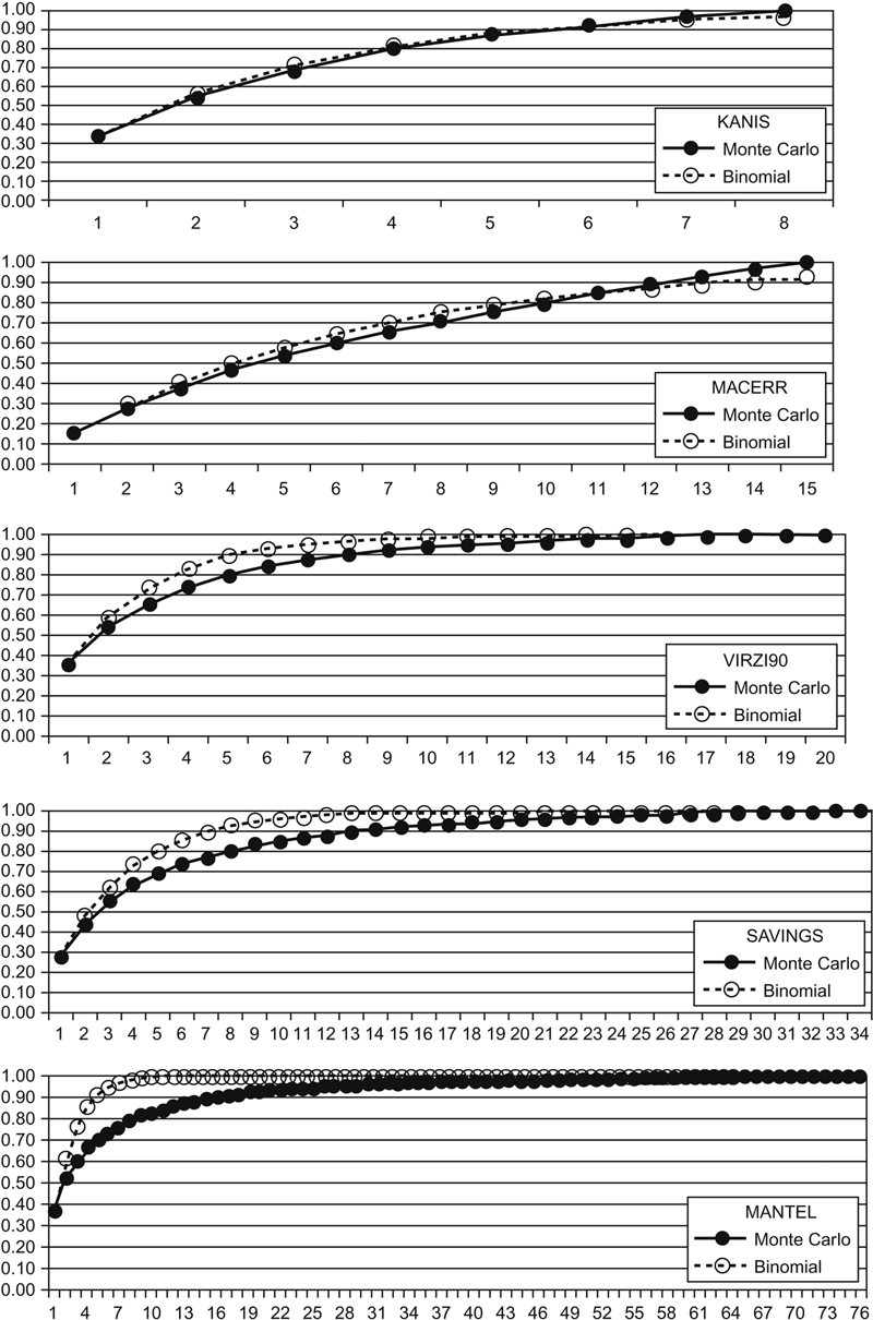
Figure 7.6 Monte Carlo and Binomial Problem Discovery Curves for Five Usability Evaluations.
Table 7.9
Analyses of Maximum Differences Between Monte Carlo and Binomial Models for Five Usability Evaluations
| Database/Type of Evaluation | Total Sample Size | Total Number of Problems Discovered | Max Difference (Proportion) | Max Difference (Number of Problems) | At n = | p |
| KANIS (Usability Test) | 8 | 22 | 0.03 | 0.7 | 3 | 0.35 |
| MACERR (Usability Test) | 15 | 145 | 0.05 | 7.3 | 6 | 0.16 |
| VIRZI90 (Usability Test) | 20 | 40 | 0.09 | 3.6 | 5 | 0.36 |
| SAVINGS (Heuristic Evaluation) | 34 | 48 | 0.13 | 6.2 | 7 | 0.26 |
| MANTEL (Heuristic Evaluation) | 76 | 30 | 0.21 | 6.3 | 6 | 0.38 |
| Mean | 30.6 | 57.0 | 0.102 | 4.8 | 5.4 | 0.302 |
| Std Dev | 27.1 | 50.2 | 0.072 | 2.7 | 1.5 | 0.092 |
| N Studies | 5 | 5 | 5 | 5 | 5 | 5 |
| sem | 12.1 | 22.4 | 0.032 | 1.2 | 0.7 | 0.041 |
| df | 4 | 4 | 4 | 4 | 4 | 4 |
| t-crit-90 | 2.13 | 2.13 | 2.13 | 2.13 | 2.13 | 2.13 |
| d-crit-90 | 25.8 | 47.8 | 0.068 | 2.6 | 1.4 | 0.087 |
| 90% CI Upper Limit | 56.4 | 104.8 | 0.170 | 7.4 | 6.8 | 0.389 |
| 90% CI Lower Limit | 4.8 | 9.2 | 0.034 | 2.3 | 4.0 | 0.215 |

Table 7.9 shows, for this set of studies, the mean maximum deviation of the binomial from the Monte Carlo curve was 0.102 (10.2%—with 90% confidence interval ranging from 3.4% to 17.0%). Given the total number of problems discovered in the usability evaluations, the mean deviation of expected (binomial) versus observed (Monte Carlo) was 4.81 problems (with 90% confidence interval ranging from 2.3 to 7.4). The sample size at which the maximum deviation occurred (“At n =”) was, on average, 5.4 (with 90% confidence interval ranging from 4.0 to 6.8, about 4 to 7). There was a strong relationship between the magnitude of the maximum deviation and the sample size of the study (r = 0.97, 90% confidence interval ranging from 0.73 to 1.00, t(3) = 6.9, p = 0.006). The key findings are:
• The binomial model tends to overestimate the magnitude of problem discovery early in an evaluation, especially for relatively large-sample studies.
• The average sample size at which the maximum deviation occurs (in other words, the typical point of maximum over-optimism) is at the “Magic Number 5.”
• On average, however, that overestimation appears not to lead to very large discrepancies between the expected and observed numbers of problems.
To summarize, the data suggest that although violations of the assumptions of the binomial distribution do affect binomial problem-discovery models, the conclusions drawn from binomial models tend to be robust against those violations. Practitioners need to exercise care not to claim too much accuracy when using these methods, but, based on the available data, can use them with reasonable confidence.
It would be helpful to the field of usability engineering, however, to have more large-sample databases of usability problem discovery to include in analyses of problem discovery. The best model to use likely depends on different characteristics of the problem discovery databases (e.g., large or small sample size, user test or heuristic evaluation, etc.). To conduct generalizable usability research on this topic, we need more examples. Usability practitioners who have large-sample problem-discovery databases should include these matrices in their reports (using a format similar to those of Virzi, 1990, Lewis, 2001, or Kanis, 2011), and should seek opportunities for external publication in venues such as the Journal of Usability Studies. Usability researchers should include any new problem discovery databases as appendices in their journal articles.
This type of research is interesting and important (at least, we think so), but it is also important not to lose sight of the practical aspects of formative user research, which is based on rapid iteration with small samples (Barnum et al., 2003; Lewis, 2012; Nielsen, 2000). This practical consideration lies at the heart of iterative test and redesign, for example, as expressed by Medlock et al. (2005, p. 489) in their discussion of the Rapid Iterative Test and Evaluation (RITE) method:
Pretend you are running a business. It is a high-risk business and you need to succeed. Now imagine two people come to your office:
• The first person says, “I’ve identified all problems we might possibly have.”
• The second person says, “I’ve identified the most likely problems and have fixed many of them. The system is measurably better than it was.”
Which one would you reward? Which one would you want on your next project? In our experience, businesses are far more interested in getting solutions than in uncovering issues.
The beta-binomial, logit-normal binomial, and capture-recapture models may turn out to provide more accurate models than the simple binomial for the discovery of events of interest in user research. This is an ongoing research topic in usability engineering, as well as in biology and software engineering. Time (and more Monte Carlo studies) will tell. For now, however, the most practical approach is to use the simple method taught at the beginning of this chapter unless it is mission critical to have a very precise estimate of the number of events available for discovery and the number of undiscovered events, in which case the usability testing team should include a statistician with a background in advanced discovery modeling.
Most usability practitioners do not need this level of precision in their day-to-day work. In fact, using the basic method (see Section “Using a Probabilistic Model of Problem Discovery to Estimate Sample Sizes for Formative User Research” at the beginning of this chapter), there is no need to attempt to compute any composite estimate of p or the number of undiscovered problems, thus avoiding the more complex issues discussed in the remainder of the chapter. This is analogous to the observation of Dorazio and Royle (2003) in their discussion of estimating the size of closed populations of animals (p. 357):
Generally, we expect the MLE [maximum likelihood estimate] to perform better as the proportion of the population that is observed in a sample increases. The probability that a single individual detected with probability p is observed at least once in T capture occasions is 1 – (1 – p)T. Therefore, it is clear that increasing T is expected to increase the proportion of the population that is observed, even in situations where individual capture rates p are relatively small. In many practical problems T may be the only controllable feature of the survey, so it is important to consider the impact of T on the MLE’s performance.
Key points
• The purpose of formative user research is to discover and enumerate the events of interest in the study (e.g., the problems that participants experience during a formative usability study).
• The most commonly used discovery model in user research is P(x ≥ 1) = 1 – (1 – p)n, derived from the binomial probability formula.
• The sample size formula based on this equation is n = ln(1 – P(x > 1))/ln(1 – p), where P(x > 1) is the discovery goal, p is the target probability of the events of interest under study (for example, the probability of a usability problem occurring during a formative usability test), and ln means to take the natural logarithm.
• To avoid issues associated with estimates of p averaged across a set of problems or participants (which violates the homogeneity assumption of the binomial model), set p equal to the smallest level that you want to be able to discover (so you are setting rather than estimating the value of p).
• If you are willing to take some risk of overestimating the effectiveness of your research when n is small (especially in the range of n = 4–7), you can estimate p by averaging across a set of observed problems and participants.
• If this estimate comes from a small-sample study, then it is important to adjust the initial estimate of p (using the third formula in Table 7.10 below).
• For small values of p (around 0.10), a reasonable discovery goal is about 86%; for p between 0.25 and 0.50, the goal should be about 98%; for p between 0.10 and 0.25, interpolate.
• Note that the sample sizes for these goals are total sample sizes—the target sample size per iteration should be roughly equal to the total sample size divided by the planned number of iterations—if not equal, then use smaller sample sizes at the beginning of the study for more rapid iteration in the face of discovery of higher-probability events.
• You can use the adjusted estimate of p to roughly estimate the number of events of interest available for discovery and the number of undiscovered events.
• The limited data available indicates that even with the overestimation problem, the discrepancies between observed and expected numbers of problems are not large.
• Alternative models may provide more accurate estimation of problem discovery based on averages across problems or participants, but requires more complex modeling, so if a mission-critical study requires very high precision of these estimates, the team should include a statistician with a background in discovery modeling.
• Table 7.10 provides a list of the key formulas discussed in this chapter.
Table 7.10
List of Sample Size Formulas for Formative Research
| Name of Formula | Formula | Notes |
The famous equation: 1 – (1 – p)n |
|
Computes the likelihood of seeing events of probability p at least once with a sample size of n—derived by subtracting the probability of 0 occurrences (binomial probability formula) from 1 |
| Sample size for formative research |
|
The equation above, solved for n—to use, set P(x > 1) to a discovery goal (for example, 0.85 for 85%) and p to the smallest probability of an event that you are interested in detecting in the study—ln stands for “natural logarithm” |
| Combined adjustment for small-sample estimates of p |

|
From Lewis (2001)—two-component adjustment combining deflation and Good-Turing discounting: pest is the estimate of p from the observed data; GTadj is the number of problem types observed only once divided by the total number of problem types |
| Quick adjustment formula |
|
Regression equation based on 19 usability studies—to use when problem-by-participant matrix not available |
| Binomial probability formula |

|
Probability of seeing exactly x events of probability p with n trials |

..................Content has been hidden....................
You can't read the all page of ebook, please click here login for view all page.